Alert - This a masked version for internal use only
4. Supplementary Analyses
Load Data
Code
load("../data/wrangled_data/dt_items.RData")dt_cfa <- dt_items %>%select(-response_id,-age,-religion,-education,-gender,-starts_with("intuition"),-starts_with("logic"),-starts_with("past_activism") # not really a scale ) %>%filter(country !="Jihadist") # fit statistics get calculated differently due to binary nature of scales
Code
impute_items =FALSEif (impute_items) { res <-impute_flex( dt_cfa, # your other datasetscope ="all", # <- this is the new modeid_vars =c("response_id"), # protect all ID-like columns# never_impute_extra = c("created_at"), # optionally protect extra columnsm =20,maxit =10,seed =42,verbose =TRUE,parallel_mode ="cluster", # <— turn on cluster backendcores = parallel::detectCores() -2,cl_type =if (.Platform$OS.type =="windows") "PSOCK"else"FORK" ) dt_cfa <- res$completed}
# Get the unique list of countries for all analysesunique_countries <-unique(dt_cfa$country)unique_models <-unique(names(cfa_models))
Invariance
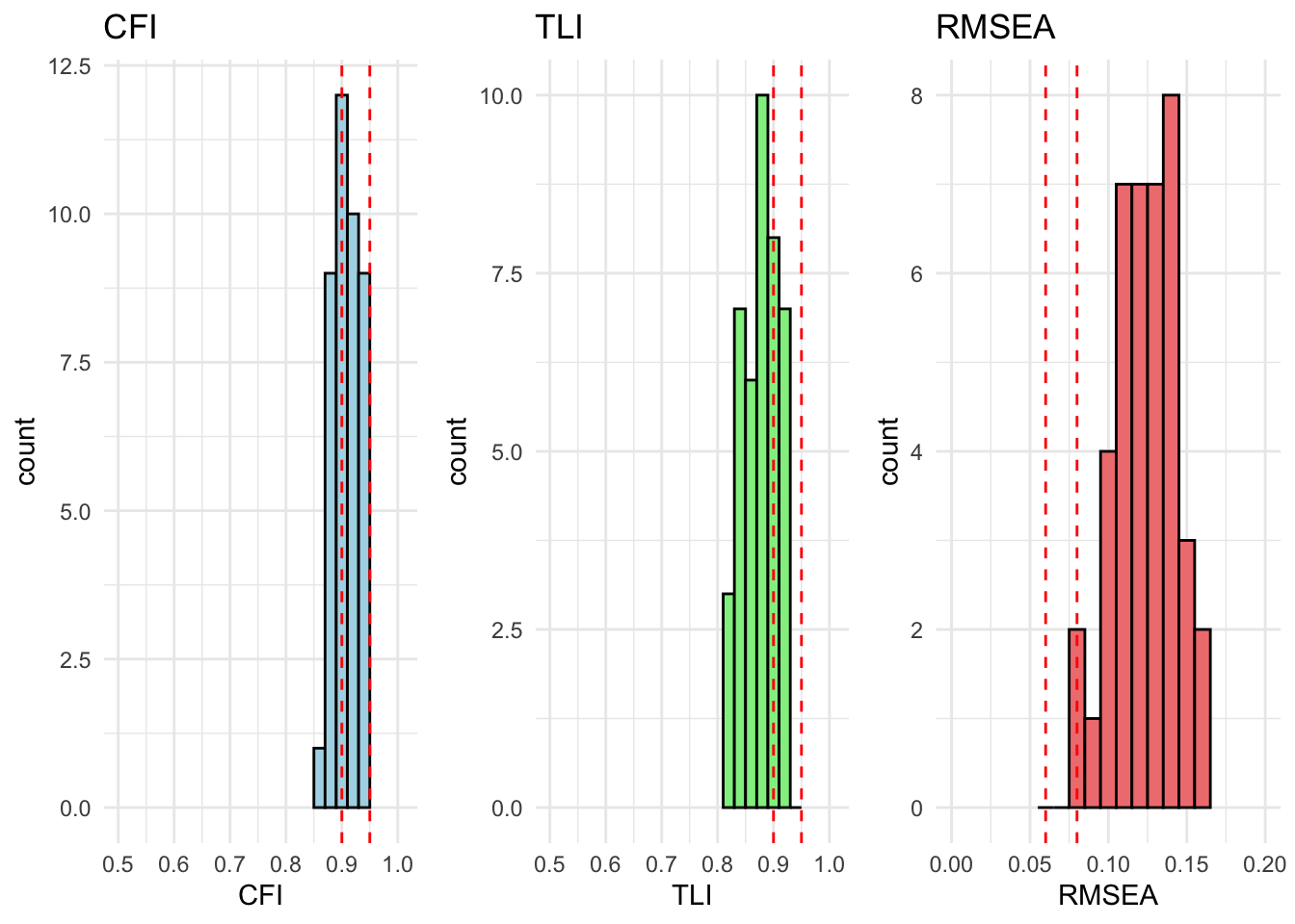
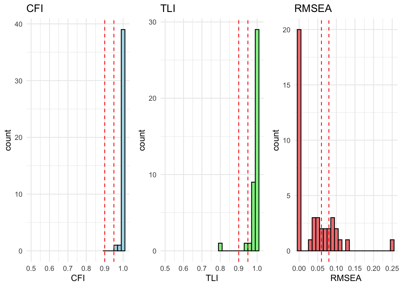
Configurial Invariance
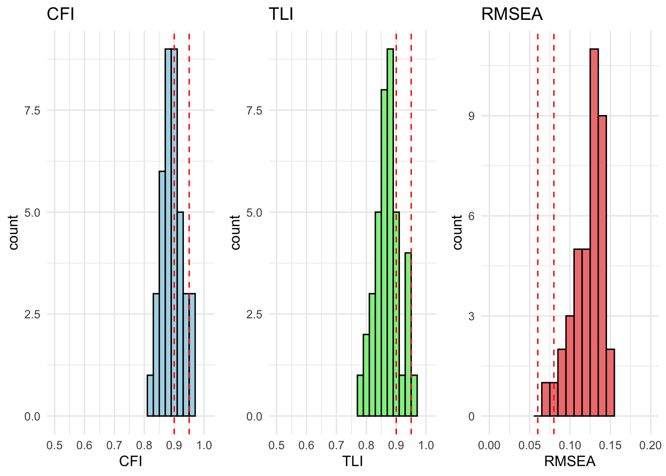
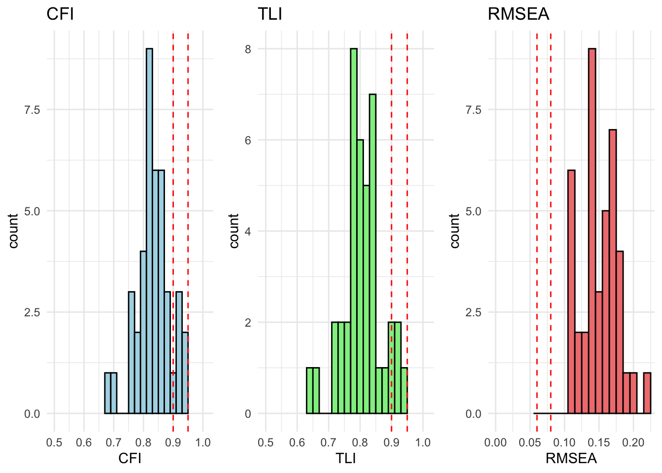
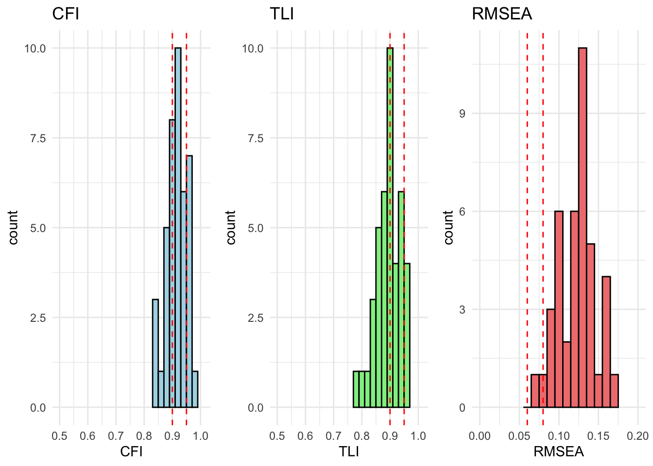
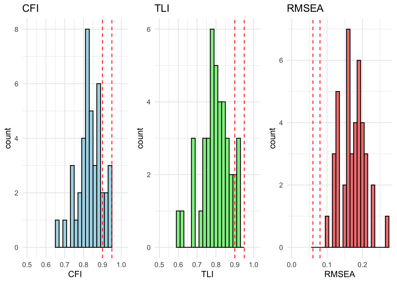
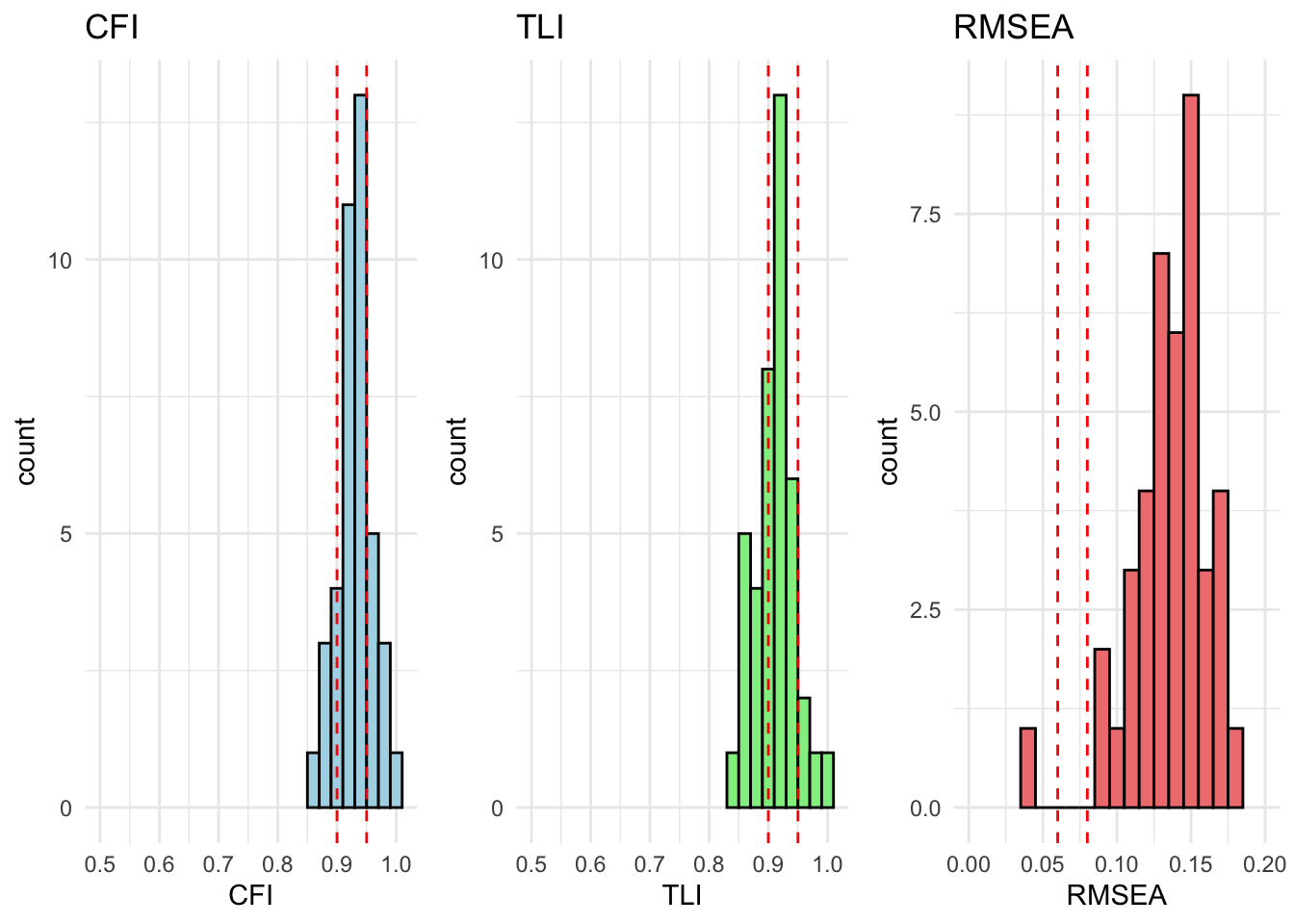
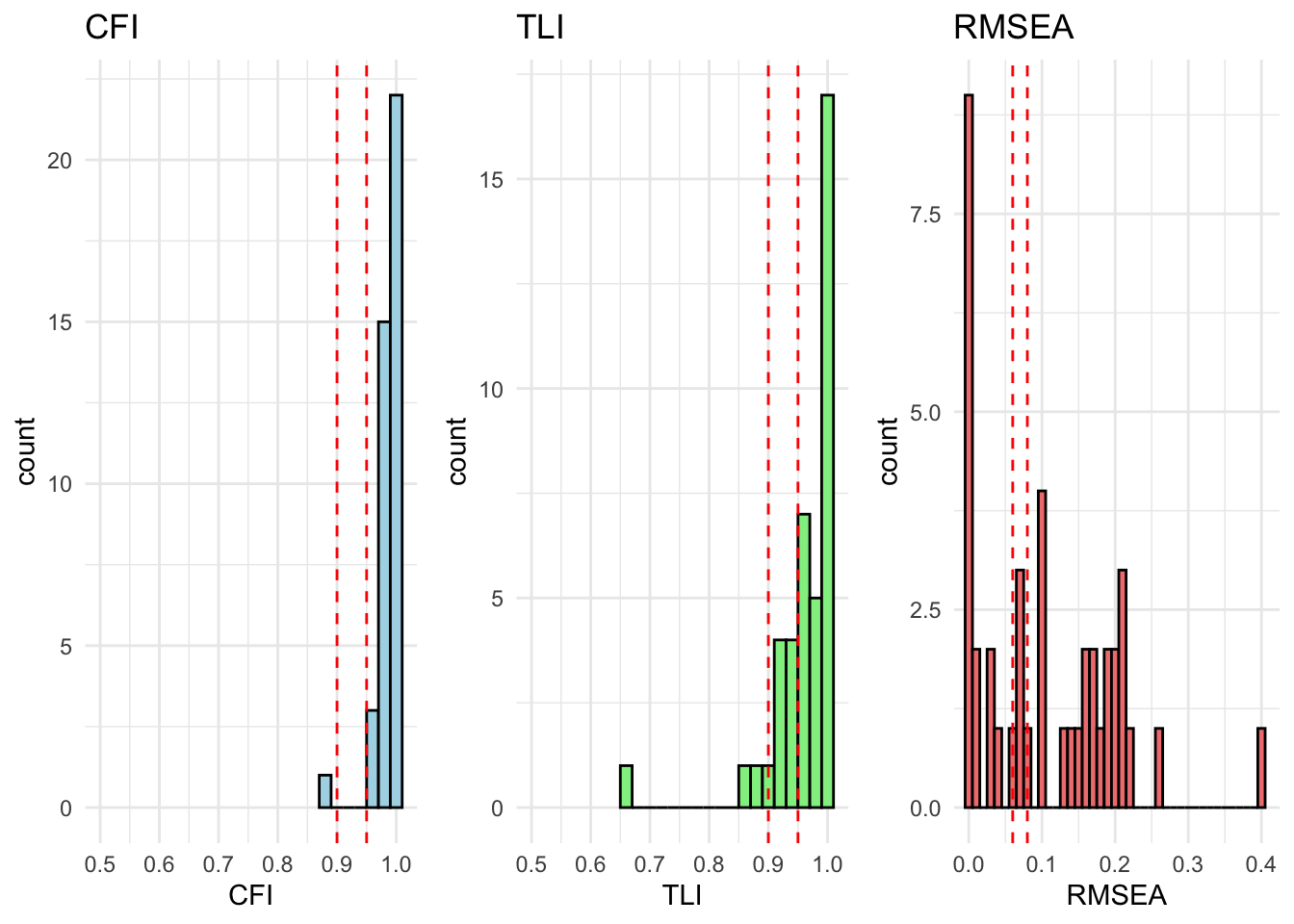
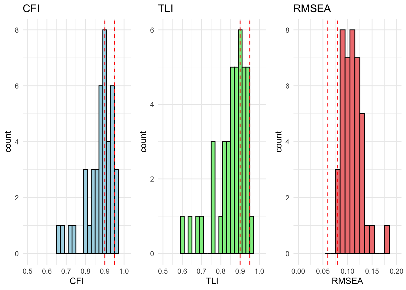
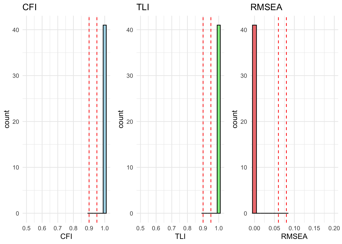
Configural invariance is the most basic level of invariance, where the same factor structure is assumed across groups, but the parameters (loadings, intercepts, etc.) are allowed to vary. Individual model fit can be found in the model comparison section.
# build a tidy summary once# result_fit_configural_df <- collect_fit_summary(fit_configural)# # # Use the model names present in the results/summaries# unique_models <- unique(result_fit_configural_df$model)# # for (model in unique_models) {# # node <- get_result_node(fit_configural, model, tag = "Grouped")# if (is.null(node)) next# # mi_tbl <- get_mod_indices_tbl(node)# show_output <- should_show(node, mi_tbl)# # if (show_output) {# h4(paste("Model:", model))# # if (!isTRUE(node$converged)) {# cat("This model did <b>not converge</b> — review identification, starting values, or data quality.<br>")# } else if (nrow(mi_tbl) >= 1) {# cat("This model shows <b>inadequate fit</b> (low CFI/TLI or flagged MIs).<br>")# } else {# cat("Model converged without flagged modification indices.<br>")# }# # # Overall fit stats (from the tidy summary)# print_fit_table(result_fit_configural_df, model)# # # Modification indices (if any)# if (nrow(mi_tbl) >= 1) {# cat("<br>Top modification indices (first 5 shown):<br>")# # If you want only the same top-5 as computed, mi_tbl already reflects that.# kable(mi_tbl,# caption = sprintf("Modification indices for %s", model)) |># kable_styling(full_width = FALSE, latex_options = c("hold_position", "scale_down")) |># print()# }# }# }# extract relevant stats# result_fit_configural_df <- extract_fit_statistics_from_results(fit_configural)# # # runng above function over models# for (model in unique_models) {# # # if there are no modification indices, the model fits well# mod_indices <- fit_configural[[model]][["Grouped_Countries"]]$mod_indices %>% as_tibble() %>% mutate_if(is.numeric, round, 2)# # only show output if model does not fit (there are no rows)# show_output <- nrow(mod_indices) > 1# # if (show_output) {# cat("<br><h4>Model:", model, "</h4><br>")# cat("This model has inadequate fit.<br>")# cat("Overall fit statistics:<br>")# # visualize_individual_fit_statistics(# df = result_fit_configural_df, # cfa_model = model# )# # cat("Modification indices:<br>")# mod_indices %>% # kable(., caption = paste("Modification indices for", model)) %>%# kable_styling(full_width = F, latex_options = c("hold_position", "scale-down")) %>% # print()# }# }# fit_configural <- sem(cfa_model_intent, data = dt_cfa, group = "country", optim.method = "nlminb")# fit_configural <- sem(cfa_model_intent, data = dt_cfa, group = "country", optim.method = "em", verbose = T,# em.iter.max = 20000, em.fx.tol = 1e-08, em.dx.tol = 1e-04)
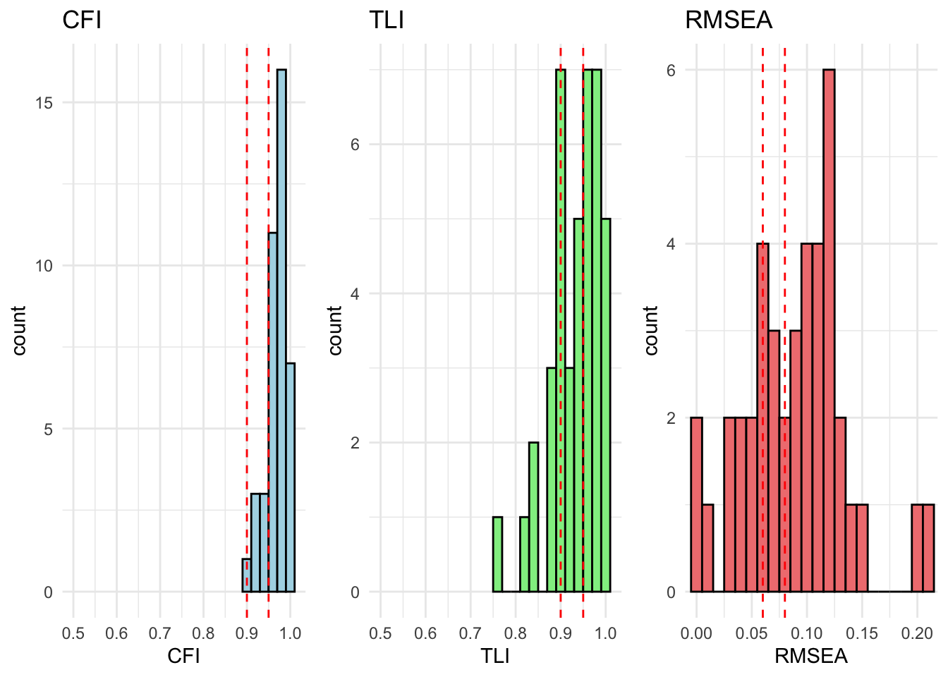
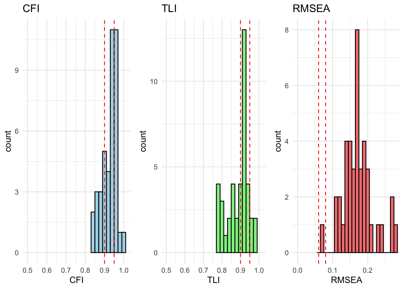
Metric Invariance
Metric invariance constrains the factor loadings to be equal across groups. Individual model fit can be found in the model comparison section.
# extract relevant stats# result_fit_metric_df <- extract_fit_statistics_from_results(fit_metric)# # # runng above function over models# for (model in unique_models) {# # # if there are no modification indices, the model fits well# mod_indices <- fit_metric[[model]][["Grouped_Countries"]]$mod_indices %>% as_tibble() %>% mutate_if(is.numeric, round, 2)# # only show output if model does not fit (there are no rows)# show_output <- nrow(mod_indices) > 1# # if (show_output) {# cat("<br><h4>Model:", model, "</h4><br>")# cat("This model has inadequate fit.<br>")# cat("Overall fit statistics:<br>")# # visualize_individual_fit_statistics(# df = result_fit_metric_df, # cfa_model = model# )# # cat("Modification indices:<br>")# mod_indices %>% # kable(., caption = paste("Modification indices for", model)) %>%# kable_styling(full_width = F, latex_options = c("hold_position", "scale-down")) %>% # print()# }# }
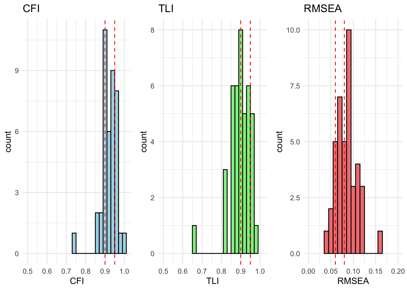
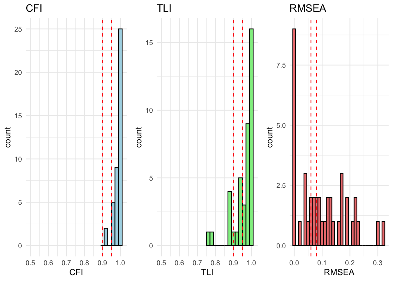
Scalar Invariance
Scalar invariance involves constraining both the factor loadings and the intercepts to be equal across groups. Individual model fit can be found in the model comparison section.
# extract relevant stats# result_fit_scalar_df <- extract_fit_statistics_from_results(fit_scalar)# # # runng above function over models# # runng above function over models# for (model in unique_models) {# # # if there are no modification indices, the model fits well# mod_indices <- fit_scalar[[model]][["Grouped_Countries"]]$mod_indices %>% as_tibble() %>% mutate_if(is.numeric, round, 2)# # only show output if model does not fit (there are no rows)# show_output <- nrow(mod_indices) > 1# # if (show_output) {# cat("<br><h4>Model:", model, "</h4><br>")# cat("This model has inadequate fit.<br>")# cat("Overall fit statistics:<br>")# # visualize_individual_fit_statistics(# df = result_fit_scalar_df, # cfa_model = model# )# # cat("Modification indices:<br>")# mod_indices %>% # kable(., caption = paste("Modification indices for", model)) %>%# kable_styling(full_width = F, latex_options = c("hold_position", "scale-down")) %>% # print()# }# }
Model Comparison
We can compare models using a chi-square difference test or by comparing fit indices like CFI and RMSEA. Our main comparison of interest is configural to metric invariance. This is because we are mainly interested in whether the relationship between the items and the underlying latent variable as well as the relationships between the variables remain constant. Intercepts and mean comparisons are not the focus of this analysis. Our main statistic of interference are TLI and CFI. RMSEA and the Chi-quared will most likely be heavily influences by the large sample size.
# Initialize the model_descriptions list with unique_models as namesmodel_descriptions <-setNames(vector("list", length(unique_models)), unique_models)# describe the individual modelsmodel_descriptions[["cfa_model_intent"]] <-"Cross-cultural performance of the violent and peaceful intent scales is satisfactory. TLI and CFI remain stable despite increasing model restrictions."model_descriptions[["cfa_model_radical_attitudes"]] <-"A just-identified three-item, one-factor CFA shows strong item loadings across countries. Due to the just-identified nature, TLI and CFI at 1. We are using the default lavaan <i>marker method</i> which fixes the first loading to 1."model_descriptions[["cfa_model_passion"]] <-"Initial model fit is suboptimal; cross-country data is not ideal.<br><b>After checking:</b><br>We adjusted one residual covariance (commitment_passion_14 ~~ commitment_passion_15) which improved model fit to an acceptable level."model_descriptions[["cfa_model_passion_core"]] <-"Model fit is acceptable. The commitment scale is often seen as a seperate entity (measuring the presence of passion) which is why we also tested it seperately."model_descriptions[["cfa_model_commitment_passion"]] <-"Seperating this from the original three factor solution improved model fit substantially. Adjusting one parameter increased model fit dramatically (commitment_passion_14 ~~ commitment_passion_15). Either the original scale or the seperation suggest an acceptable model solution."model_descriptions[["cfa_model_identity_fusion"]] <-"Configural and metric invariance are supported, but scalar invariance is weak. Avoid comparing intercepts or means across countries."model_descriptions[["cfa_model_ingroup_superiority"]] <-"The ingroup superiority scale demonstrates good model fit even under scalar invariance."model_descriptions[["cfa_model_collective_relative_deprivation"]] <-"Configural and metric invariance are defensible; scalar invariance is uncertain. Avoid comparing intercepts or means across countries."model_descriptions[["cfa_model_perceived_discrimination"]] <-"Good model fit. TLI and CFI fit indices remain above thresholds across restrictive models."model_descriptions[["cfa_model_activist_intent"]] <-"Good model fit across countries, including under more restrictive conditions."model_descriptions[["cfa_model_moral_neutralization"]] <-"Model fit is poor; data from Argentina, Denmark, and Colombia did not converge.<br><b>After checking:</b> We cannot assume scalar invariance. However, both configural and metric invariance are in line with [previous implementations of invariance](https://www.researchgate.net/publication/279472182_Are_Moral_Disengagement_Neutralization_Techniques_and_Self-Serving_Cognitive_Distortions_the_Same_Developing_a_Unified_Scale_of_Moral_Neutralization_of_Aggression). As not our core variable, we use it as a variable in the random forest but cross-cultural conclusions regarding the variable should be drawn cautiously."model_descriptions[["cfa_model_anger"]] <-"Model fit is bad. While all countries converge, the fit within each country is not satisfactory.<br><b>After checking:</b><br>Adjusting the following residual covariances improved model fit (anger_9 ~~ anger_10; anger_1 ~~ anger_2)."model_descriptions[["cfa_model_anger_one_fac"]] <-"This is the original scale without the adjusted items. Adjusting two residual covariances resulted in satisfactory model fit (anger_1 ~~ anger_2; anger_6 ~~ anger_7)."model_descriptions[["cfa_model_affect"]] <-"Configural and metric invariance are marginal; scalar invariance is not supported. Fit within individual countries is generally satisfactory, but conclusions should be cautious."# Print results for each modelfor (model in unique_models) {cat("<br><h4>Model:", model, "</h4><br>")# Print the description for the current model description <- model_descriptions[[model]]if (!is.null(description) && description !="") {cat("Description:<br>", description, "<br>") } else {cat("<p>No description available for this model.</p><br>") } anova_results[[model]] %>%kable(., caption =paste("ANOVA Model comparison for", model)) %>%kable_styling(full_width = F, latex_options =c("hold_position", "scale-down")) %>%print()}
Model: cfa_model_intent
Description: Cross-cultural performance of the violent and peaceful intent scales is satisfactory. TLI and CFI remain stable despite increasing model restrictions.
ANOVA Model comparison for cfa_model_intent
name
Df
AIC
BIC
Chisq
Chisq diff
RMSEA
Df diff
Pr(>Chisq)
TLI
CFI
rmsea
configural
1763
369641.4
379737.4
10275.95
NA
NA
NA
NA
0.904
0.925
0.138
metric
2123
369861.6
377350.4
11216.19
940.2403
0.0799940
360
0
0.915
0.920
0.130
scalar
2483
372778.0
377659.4
14852.55
3636.3641
0.1900858
360
0
0.901
0.891
0.141
Model: cfa_model_passion
Description: Initial model fit is suboptimal; cross-country data is not ideal. After checking: We adjusted one residual covariance (commitment_passion_14 ~~ commitment_passion_15) which improved model fit to an acceptable level.
ANOVA Model comparison for cfa_model_passion
name
Df
AIC
BIC
Chisq
Chisq diff
RMSEA
Df diff
Pr(>Chisq)
TLI
CFI
rmsea
configural
4100
521264.4
536705.4
19911.66
NA
NA
NA
NA
0.878
0.898
0.124
metric
4620
522073.0
533748.0
21760.31
1848.654
0.1007185
520
0
0.882
0.890
0.121
scalar
5140
528092.8
536001.6
28820.04
7059.734
0.2234515
520
0
0.854
0.848
0.135
Model: cfa_model_passion_one_factor
No description available for this model.
ANOVA Model comparison for cfa_model_passion_one_factor
name
Df
AIC
BIC
Chisq
Chisq diff
RMSEA
Df diff
Pr(>Chisq)
TLI
CFI
rmsea
configural
4223
530564.0
545114.2
29457.29
NA
NA
NA
NA
0.811
0.837
0.154
metric
4823
532143.3
542348.0
32236.57
2779.279
0.1200841
600
0
0.820
0.823
0.150
scalar
5423
541164.5
547023.7
42457.76
10221.188
0.2523153
600
0
0.784
0.761
0.165
Model: cfa_model_passion_core
Description: Model fit is acceptable. The commitment scale is often seen as a seperate entity (measuring the presence of passion) which is why we also tested it seperately.
ANOVA Model comparison for cfa_model_passion_core
name
Df
AIC
BIC
Chisq
Chisq diff
RMSEA
Df diff
Pr(>Chisq)
TLI
CFI
rmsea
configural
2173
397469.3
408456.2
10887.57
NA
NA
NA
NA
0.900
0.920
0.126
metric
2573
397758.6
405848.5
11976.86
1089.290
0.0827134
400
0
0.909
0.913
0.120
scalar
2973
401469.3
406662.2
16487.57
4510.703
0.2019914
400
0
0.887
0.875
0.134
Model: cfa_model_passion_core_one_factor
No description available for this model.
ANOVA Model comparison for cfa_model_passion_core_one_factor
name
Df
AIC
BIC
Chisq
Chisq diff
RMSEA
Df diff
Pr(>Chisq)
TLI
CFI
rmsea
configural
2214
406104.2
416794.2
19604.46
NA
NA
NA
NA
0.804
0.840
0.177
metric
2654
407268.3
414771.6
21648.56
2044.095
0.1203077
440
0
0.821
0.825
0.169
scalar
3094
413581.0
417897.5
28841.22
7192.660
0.2468402
440
0
0.792
0.763
0.182
Model: cfa_model_commitment_passion
Description: Seperating this from the original three factor solution improved model fit substantially. Adjusting one parameter increased model fit dramatically (commitment_passion_14 ~~ commitment_passion_15). Either the original scale or the seperation suggest an acceptable model solution.
ANOVA Model comparison for cfa_model_commitment_passion
name
Df
AIC
BIC
Chisq
Chisq diff
RMSEA
Df diff
Pr(>Chisq)
TLI
CFI
rmsea
configural
41
138249.3
142109.5
73.28548
NA
NA
NA
NA
0.992
0.999
0.056
metric
161
138819.9
141811.0
883.91621
810.6307
0.1511674
120
0
0.956
0.971
0.134
scalar
281
140828.9
142951.0
3132.96336
2249.0471
0.2654165
120
0
0.901
0.887
0.201
Model: cfa_model_identity_fusion
Description: Configural and metric invariance are supported, but scalar invariance is weak. Avoid comparing intercepts or means across countries.
ANOVA Model comparison for cfa_model_identity_fusion
name
Df
AIC
BIC
Chisq
Chisq diff
RMSEA
Df diff
Pr(>Chisq)
TLI
CFI
rmsea
configural
574
228001.9
234237.6
5158.894
NA
NA
NA
NA
0.896
0.931
0.178
metric
814
228286.0
232783.6
5923.020
764.1262
0.0931190
240
0
0.919
0.923
0.158
scalar
1054
231891.8
234651.1
10008.741
4085.7204
0.2522372
240
0
0.890
0.865
0.184
Model: cfa_model_ingroup_superiority
Description: The ingroup superiority scale demonstrates good model fit even under scalar invariance.
ANOVA Model comparison for cfa_model_ingroup_superiority
name
Df
AIC
BIC
Chisq
Chisq diff
RMSEA
Df diff
Pr(>Chisq)
TLI
CFI
rmsea
configural
82
144400.8
147964.1
445.8304
NA
NA
NA
NA
0.957
0.986
0.133
metric
202
144379.4
147073.5
664.3759
218.5456
0.0571023
120
1e-07
0.978
0.982
0.095
scalar
322
145517.8
147342.9
2042.8221
1378.4462
0.2040575
120
0e+00
0.948
0.932
0.146
Model: cfa_model_collective_relative_deprivation
Description: Configural and metric invariance are defensible; scalar invariance is uncertain. Avoid comparing intercepts or means across countries.
ANOVA Model comparison for cfa_model_collective_relative_deprivation
name
Df
AIC
BIC
Chisq
Chisq diff
RMSEA
Df diff
Pr(>Chisq)
TLI
CFI
rmsea
configural
369
216139.8
221484.7
1861.817
NA
NA
NA
NA
0.934
0.961
0.127
metric
569
216291.6
220188.0
2413.636
551.8185
0.0835698
200
0
0.947
0.951
0.113
scalar
769
218198.5
220646.5
4720.559
2306.9235
0.2045098
200
0
0.917
0.896
0.143
Model: cfa_model_perceived_discrimination
Description: Good model fit. TLI and CFI fit indices remain above thresholds across restrictive models.
ANOVA Model comparison for cfa_model_perceived_discrimination
name
Df
AIC
BIC
Chisq
Chisq diff
RMSEA
Df diff
Pr(>Chisq)
TLI
CFI
rmsea
configural
1804
271619.0
281418.1
10591.81
NA
NA
NA
NA
0.917
0.933
0.139
metric
2204
272045.5
278947.6
11818.31
1226.501
0.0905725
400
0
0.926
0.927
0.132
scalar
2604
273087.7
277092.8
13660.51
1842.194
0.1196429
400
0
0.927
0.916
0.130
Model: cfa_model_activist_intent
Description: Good model fit across countries, including under more restrictive conditions.
ANOVA Model comparison for cfa_model_activist_intent
name
Df
AIC
BIC
Chisq
Chisq diff
RMSEA
Df diff
Pr(>Chisq)
TLI
CFI
rmsea
configural
82
137553.4
141116.7
491.9483
NA
NA
NA
NA
0.961
0.987
0.141
metric
202
137585.1
140279.3
763.6385
271.6902
0.0708424
120
0
0.979
0.982
0.105
scalar
322
138430.2
140255.4
1848.7896
1085.1511
0.1786948
120
0
0.963
0.952
0.137
Model: cfa_model_moral_neutralization
Description: Model fit is poor; data from Argentina, Denmark, and Colombia did not converge. After checking: We cannot assume scalar invariance. However, both configural and metric invariance are in line with previous implementations of invariance. As not our core variable, we use it as a variable in the random forest but cross-cultural conclusions regarding the variable should be drawn cautiously.
ANOVA Model comparison for cfa_model_moral_neutralization
name
Df
AIC
BIC
Chisq
Chisq diff
RMSEA
Df diff
Pr(>Chisq)
TLI
CFI
rmsea
configural
4264
490548.2
504800.7
17793.51
NA
NA
NA
NA
0.877
0.894
0.112
metric
4864
491448.5
501355.7
19893.79
2100.279
0.0996551
600
0
0.881
0.882
0.111
scalar
5464
497480.8
503042.8
27126.10
7232.310
0.2095298
600
0
0.847
0.830
0.125
Model: cfa_model_radical_attitudes
Description: A just-identified three-item, one-factor CFA shows strong item loadings across countries. Due to the just-identified nature, TLI and CFI at 1. We are using the default lavaan marker method which fixes the first loading to 1.
ANOVA Model comparison for cfa_model_radical_attitudes
name
Df
AIC
BIC
Chisq
Chisq diff
RMSEA
Df diff
Pr(>Chisq)
TLI
CFI
rmsea
configural
0
90231.46
92903.94
0.0000
NA
NA
NA
NA
1.000
1.000
0.000
metric
80
90380.36
92473.45
308.9032
308.9032
0.1065825
80
0.0e+00
0.988
0.992
0.107
scalar
160
90369.62
91883.30
458.1618
149.2587
0.0586269
80
4.3e-06
0.992
0.990
0.086
Model: cfa_model_anger
Description: Model fit is bad. While all countries converge, the fit within each country is not satisfactory. After checking: Adjusting the following residual covariances improved model fit (anger_9 ~~ anger_10; anger_1 ~~ anger_2).
ANOVA Model comparison for cfa_model_anger
name
Df
AIC
BIC
Chisq
Chisq diff
RMSEA
Df diff
Pr(>Chisq)
TLI
CFI
rmsea
configural
1353
304745.0
314246.4
6692.273
NA
NA
NA
NA
0.878
0.910
0.125
metric
1713
304819.8
311714.1
7487.110
794.8372
0.0692697
360
0
0.895
0.903
0.116
scalar
2073
307090.0
311377.3
10477.335
2990.2245
0.1703634
360
0
0.874
0.859
0.127
Model: cfa_model_anger_one_fac
Description: This is the original scale without the adjusted items. Adjusting two residual covariances resulted in satisfactory model fit (anger_1 ~~ anger_2; anger_6 ~~ anger_7).
ANOVA Model comparison for cfa_model_anger_one_fac
name
Df
AIC
BIC
Chisq
Chisq diff
RMSEA
Df diff
Pr(>Chisq)
TLI
CFI
rmsea
configural
287
195772.9
201711.3
1005.769
NA
NA
NA
NA
0.929
0.967
0.100
metric
487
195778.1
200268.1
1410.923
405.1532
0.0638345
200
0
0.946
0.957
0.087
scalar
687
197240.5
200282.2
3273.396
1862.4739
0.1817161
200
0
0.893
0.881
0.122
Model: cfa_model_affect
Description: Configural and metric invariance are marginal; scalar invariance is not supported. Fit within individual countries is generally satisfactory, but conclusions should be cautious.
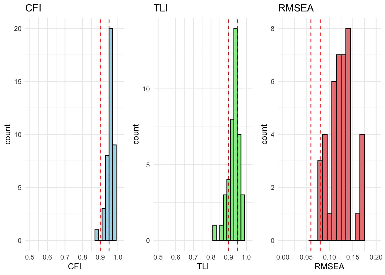
 All countries are within acceptable fit for cfa_model_radical_attitudes