3. Main Analyses

Load Data

Code
# load data for cor plots
load("../data/wrangled_data/dt_ana_violent.RData")
load("../data/wrangled_data/dt_ana_peaceful.RData")

# load CRF function
source("../scripts/functions/crf.R")
source("../scripts/functions/crf-explanations-and-labels.R")
source("../scripts/functions/supportive-functions.R")
source("../scripts/functions/fun-panel.R")

code_folder_name <- "rad-att-removed/"

# set the python variables
python_run = FALSE

python_file_raw <- paste0("code-", code_folder_name, "03-main-analysis-python-raw.py")
python_file_cw <- paste0("code-", code_folder_name, "03-main-analysis-python-cw.py")
python_file_gmc <- paste0("code-", code_folder_name, "03-main-analysis-python-gmc.py")

run_python_raw <- FALSE
run_python_cw <- FALSE
run_python_gmc <- FALSE

# set the R variables
R_run = FALSE
R_file_raw <- paste0("code-", code_folder_name, "03-main-analysis-raw.R")
R_file_cw <- paste0("code-", code_folder_name, "03-main-analysis-cw.R")
R_file_gmc <- paste0("code-", code_folder_name, "03-main-analysis-gmc.R")

run_R_raw <- FALSE
run_R_cw <- FALSE
run_R_gmc <- FALSE

run_which_R_crfs <- c(
  "ana_violent"
  # "ana_peaceful"
)

path_to_figures <- paste0("../figures/", code_folder_name)

cat(paste0("Run python analysis set to: ", python_run, "\n"))

Run python analysis set to: FALSE

Code
cat(paste0("Run R analysis set to: ", R_run, "\n"))

Run R analysis set to: FALSE

The following analyses have the radical attitudes variable removed.

Analysis

For this analysis, we are using a random forest approach: An ensemble learning method used for classification and regression that operates by constructing multiple decision trees during training. Each decision tree in the forest is built using a random subset of the data and features, which introduces diversity among the trees and helps prevent overfitting. The randomization in both data and feature selection is why the method is called a “random” forest. The individual trees are created through recursive splitting: at each node, the algorithm selects the best feature (among a random subset of features) that divides the data into two groups that are as distinct as possible with respect to the target variable (for example to predict apples, the tree may divide the data into red and other colors and realize that this was useful in distinguishing apples from other fruit; weight above 150 gram may be used for the next split –> it is always about making a TRUE vs FALSE split to separate the data better). Once all trees are built, they work together by aggregating their individual predictions, either by voting in classification tasks or averaging in regression tasks. This collective approach results in more robust and accurate predictions than a single decision tree, as the ensemble of trees helps to minimize errors and reduce variance.

Python

Code
# does not seem to work through renv so we just call the env directly!
reticulate::use_python("/Users/maximilianagostini/miniconda3/envs/extremism-predictor-project-python/bin/python")
# reticulate::py_list_packages()

# adjust python script for violent and peaceful analysis
if (python_run == TRUE) {
  tryCatch(
    {
      
      # Run the Python scripts
      if (run_python_raw) {
        cat("Running Python CRF with raw variables....\n")
        reticulate::py_run_file(python_file_raw)
      }
      
      if (run_python_cw) {
        cat("Running Python CRF with group-centered (centered within country) variables....\n")
        reticulate::py_run_file(python_file_cw)
      }
      
      if (run_python_gmc) {
        cat("Running Python CRF with grand-mean centered variables....\n")
        reticulate::py_run_file(python_file_gmc)
      }
      
    },
    error = function(e) {
      # If there's an error, print this message
      message("Could not run python script. Run in Console manually! Sometimes quarto render does not want to play! Only the plots are important so just run manually!")
    }
  )
}

R

Code
if (R_run == TRUE) {
  # specific for all crf analyses
  ntree_in <- 500
  var_imp_classic_in <- TRUE
  conditional_var_imp_classic_in <- FALSE # needs more power
  var_imp_cpi_in <- TRUE
  conditional_var_imp_cpi_in <- TRUE
  part_dep_plots_in <- FALSE
  part_dep_plots_int_in <- FALSE # use python for this
  # ice_plots_in <- FALSE
  sensitivity_in <- FALSE # use python for this
  parallel_ana_in <- TRUE
  save_output_in_memory_in <- FALSE # set to false if memory is an issue
}
Code
if (run_R_raw) {
  cat("Running R CRF with raw variables....\n")
  source(R_file_raw)
}

if (run_R_cw) {
  cat("Running R CRF with group-centered (centered within country) variables....\n")
  source(R_file_cw)
}

if (run_R_gmc) {
  cat("Running R CRF with grand-mean centered variables....\n")
  source(R_file_gmc)
}

Results

We ran a range of different analyses to test the stability of the model. Explanation:

  • Raw: Data was not centered
  • CW: Centered Within Country. For a regression analysis, we would focus on the within-country effects.
  • GMC: Grand Mean Centered For a regression analysis, we would focus on the effects across countries.

Violence

CRF

Code
# this should force the render because it needs to execute this
timestamp <- Sys.time() 

# Set path to directory containing your figures
# image_height <- "400px"  # Adjust this value as needed
dv_in = "violent_intent"

# OOB error rate
print_crf_plots(
  path_to_figures = path_to_figures,
  pattern = "OOB",
  dv_in = dv_in
)

Out of Bag Error Rate

Out of Bag (OOB) error is a method used to estimate the prediction error of Random Forest models. It leverages bootstrap sampling, where multiple subsets of the data are created by random sampling with replacement, leaving some instances out as ‘out of bag’ samples. These OOB samples provide a built-in validation set for the model, allowing error estimation without needing a separate dataset. The OOB error is calculated by aggregating predictions from trees that did not include a specific instance during training and comparing them to the actual outcomes. For an detailed description see this medium post.

Successfully read: ../figures/rad-att-removed//cw/OOB_violent_intent_python.png

Successfully read: ../figures/rad-att-removed//gmc/OOB_violent_intent_python.png

Successfully read: ../figures/rad-att-removed//raw/OOB_violent_intent_python.png

Successfully read: ../figures/rad-att-removed//cw/OOB_violent_intent.png

Successfully read: ../figures/rad-att-removed//gmc/OOB_violent_intent.png

Successfully read: ../figures/rad-att-removed//raw/OOB_violent_intent.png

Code
# variable importance FALSE
print_crf_plots(
  path_to_figures = path_to_figures,
  pattern = "varImp_FALSE",
  dv_in = dv_in
)

Variable Importance (Conditional: FALSE)

Standard variable importance plots (with conditional set to FALSE) measure the importance of a feature by assessing its contribution to prediction accuracy across all trees in a Random Forest model. This is similar to zero-order correlations but due to the tree splitting feature, other variables are still taken into account. Each feature gets permutated and the resulting drop in model accuracy is measured. The greater the decrease in accuracy, the more important the feature. The ‘null hypothesis’ is that X and Y are independent, meaning X doesn’t affect Y at all. If this is true, shuffling X won’t harm the model’s accuracy, and the importance value would be close to zero.’ (Example adjusted with help from ChatGPT from the permimp package).

Successfully read: ../figures/rad-att-removed//cw/varImp_FALSE_violent_intent_python.png

Successfully read: ../figures/rad-att-removed//gmc/varImp_FALSE_violent_intent_python.png

Successfully read: ../figures/rad-att-removed//raw/varImp_FALSE_violent_intent_python.png

Successfully read: ../figures/rad-att-removed//cw/varImp_FALSE_violent_intent.png

Successfully read: ../figures/rad-att-removed//gmc/varImp_FALSE_violent_intent.png

Successfully read: ../figures/rad-att-removed//raw/varImp_FALSE_violent_intent.png

Successfully read: ../figures/rad-att-removed//cw/varImp_CPI_FALSE_violent_intent.png

Successfully read: ../figures/rad-att-removed//gmc/varImp_CPI_FALSE_violent_intent.png

Successfully read: ../figures/rad-att-removed//raw/varImp_CPI_FALSE_violent_intent.png

Code
# variable importance TRUE
print_crf_plots(
  path_to_figures = path_to_figures,
  pattern = "varImp_TRUE",
  dv_in = dv_in
)

Variable Importance (Conditional: TRUE)

Conditional variable importance (CVI) assesses the influence of predictor variables while accounting for correlations between them. This is similar to semi-partial correlations. CVI is calculated by permuting the values of a variable and measuring the change in prediction accuracy. Compared to non-conditinoal variable importance this is done conditionally on the other variables. Example: Instead of just randomly shuffling X values across the whole dataset, you basically shuffle them according to the values in the other column. So if the other column would have two similar values, we would shuffle the values X where these values are similar. Practically, the dataset is split into smaller groups based on Z values (called a partition or grid which uses the splits made by the RF decision tree). Example adjusted with help from ChatGPT from: the permimp package)

Successfully read: ../figures/rad-att-removed//cw/varImp_CPI_TRUE_violent_intent.png

Successfully read: ../figures/rad-att-removed//gmc/varImp_CPI_TRUE_violent_intent.png

Successfully read: ../figures/rad-att-removed//raw/varImp_CPI_TRUE_violent_intent.png

Code
# variable importance
print_crf_plots(
  path_to_figures = path_to_figures,
  pattern = "partial_dep",
  dv_in = dv_in
)

Partial Dependency

Partial Dependency Plots (PDPs) show the relationship between a feature and the predicted outcome of a machine learning model, while averaging out the effects of other features. They help to visualize how a single feature influences predictions by providing an isolated view of its contribution.

Successfully read: ../figures/rad-att-removed//cw/partial_dep_violent_intent_python.png

Successfully read: ../figures/rad-att-removed//gmc/partial_dep_violent_intent_python.png

Successfully read: ../figures/rad-att-removed//raw/partial_dep_violent_intent_python.png

Code
# ICE plots
print_crf_plots(
  path_to_figures = path_to_figures,
  pattern = "ICE",
  dv_in = dv_in
)

ICE

An Individual Conditional Expectation (ICE) plot displays how a model’s predictions change for each data instance when a specific feature changes, showing a separate line for each instance. It highlights individual patterns that partial dependence plots (PDPs) might miss (A PDP is the average of the lines of an ICE plot). ICE plots are especially useful when feature interactions exist, as they uncover heterogeneous relationships between features and predictions. For an excellent explanation see Christoph Molnar’s book.

Successfully read: ../figures/rad-att-removed//cw/ICE_activist_intent_cw_violent_intent_python.png

Successfully read: ../figures/rad-att-removed//gmc/ICE_age_gmc_violent_intent_python.png

Successfully read: ../figures/rad-att-removed//raw/ICE_age_violent_intent_python.png

Successfully read: ../figures/rad-att-removed//cw/ICE_collective_relative_deprivation_cw_violent_intent_python.png

Successfully read: ../figures/rad-att-removed//gmc/ICE_collective_relative_deprivation_gmc_violent_intent_python.png

Successfully read: ../figures/rad-att-removed//raw/ICE_collective_relative_deprivation_violent_intent_python.png

Successfully read: ../figures/rad-att-removed//cw/ICE_moral_neutralization_cw_violent_intent_python.png

Successfully read: ../figures/rad-att-removed//gmc/ICE_moral_neutralization_gmc_violent_intent_python.png

Successfully read: ../figures/rad-att-removed//raw/ICE_moral_neutralization_violent_intent_python.png

Successfully read: ../figures/rad-att-removed//cw/ICE_obsessive_passion_cw_violent_intent_python.png

Successfully read: ../figures/rad-att-removed//gmc/ICE_obsessive_passion_gmc_violent_intent_python.png

Successfully read: ../figures/rad-att-removed//raw/ICE_obsessive_passion_violent_intent_python.png

Successfully read: ../figures/rad-att-removed//cw/ICE_perceived_discrimination_cw_violent_intent_python.png

Successfully read: ../figures/rad-att-removed//gmc/ICE_perceived_discrimination_gmc_violent_intent_python.png

Successfully read: ../figures/rad-att-removed//raw/ICE_perceived_discrimination_violent_intent_python.png

Code
# dt_ana_violent %>%
#   select(
#     violent_intent,
#     # radical_attitudes,
#     obsessive_passion,
#     moral_neutralization,
#     perceived_discrimination
#   ) %>%
#   pairs.panels.new()

Additional Information

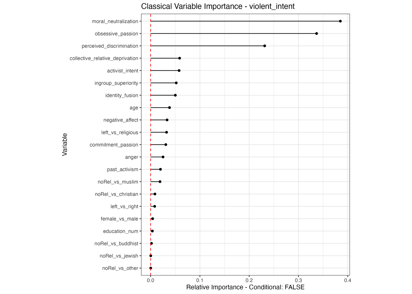
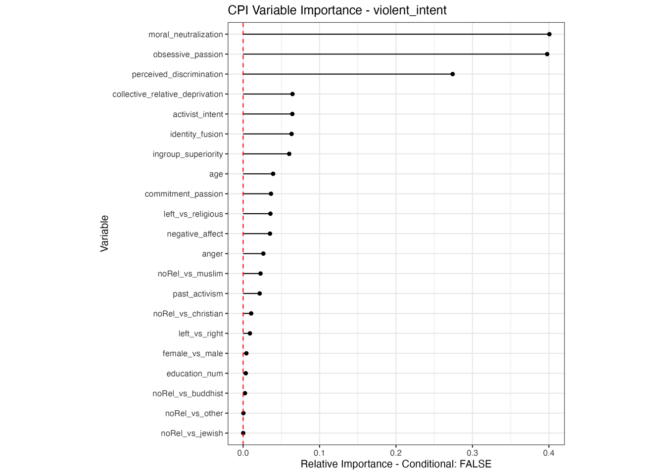
Conditional vs Unconditional Variable Importance

The following is copy-pasted from this wonderfull article. All credits go to the authors
: Debeer & Strobl, 2020.

Because there is no consensus about what variable importance is or what it should be, it is impossible to identify the true or the ideal position for a variable importance measure on this dimension. Moreover, each researcher can subjectively decide which position on the dimension — and hence which proposed importance measure — best corresponds to his or her perspective on variable importance and to the current research question.

For a simplified example, consider the situation where a pharmaceutical company has developed two new screening instruments (Test A and Test B) for assessing the presence of an otherwise hard to detect disease. A study is set up, where the two screening instruments are used on the same persons. Due to time/money restrictions, only one screening instrument can be chosen for operational use. In this case, a more marginal perspective will be the preferred option to select either Test A or Test B. For instance, the test that has the strongest association with the presence of the disease (e.g., in the spirit of a zero-order correlation) can be chosen.

In contrast, let’s assume there already is an established screening instrument (Test X), and that the pharmaceutical company has developed two new screening instruments (Test A and Test B) of which only one can be used in combination with the established instrument Test X. In this case, a more partial perspective has our preference, as it assesses the existence and strength of a contribution of either Test A or Test B on top of the established Test X. For instance, the test that shows the highest partial contribution on top of the established Test X (e.g., in the spirit of a semi-partial correlation) can be chosen to use in combination with Test X.

For an alternative example, consider a screening study on genetic determinants of a disease. A variable importance measure in the spirit of the marginal perspective would give high importance values to all genes or single-nucleotide polymorphisms (SNPs) that are associated with the disease. Each of these genes or SNPs can be useful for predicting the outbreak of the disease in future patients. A variable importance measure in the spirit of the partial perspective, however, would give high importance values to the causal genes or SNPs but lower importance to genes or SNPs associated with the causal ones due to proximity. This differentiation can be useful to generate hypotheses on the biological genesis of the disease. Hence, the question whether the marginal or partial perspective is more appropriate depends on the research question.

Important for the application to random forests
The examples does not translate one to one, because random forests are not classical models but an ensemble technique. This being said, the basic logic of conditional versus unconditional still holds up.

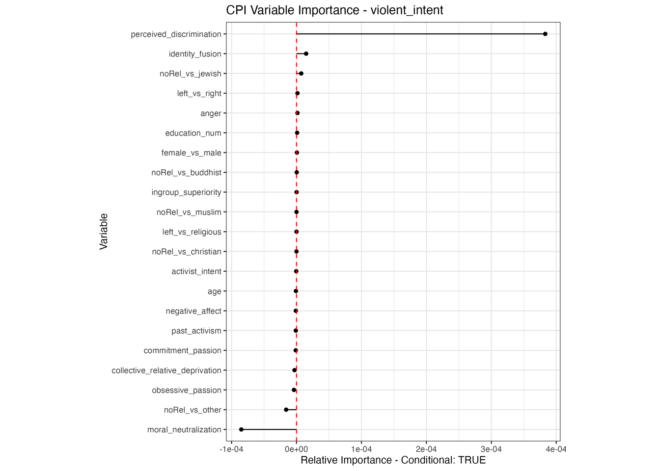
Negative values in Variable Importance plots
Interestingly, permutation variable importance can result in effects being negative. This suggests an actually improved model fit. Can be due to random Noise or Overfitting: If a predictor (X) is not really helpful for making predictions but is included in the model, it might introduce noise. When you shuffle (or permute) X, you remove the noise, and the model can make slightly better predictions. Can also be due to interaction Effects: Sometimes, a feature (X) may have complex interactions with other features (Z) in the model. When you permute X, it could disrupt these interactions in a way that ‘untangles’ some relationships in the model, leading to better performance.

References