Alert - This a masked version for internal use only
Criminal Sample Predictors via LASSO
Identifying key drivers of violent intent in the jihadi detainee data
Why a LASSO analysis?
The original random forest analysis supplied broad signals about violent intent across the wider sample. However, the criminal extremist subset is small (≈ 80 cases) and potentially idiosyncratic. LASSO regression is well-suited here because it performs feature selection and shrinkage simultaneously, guarding against overfitting in high-dimensional, low-(N) settings. The goal is to surface a compact, interpretable set of predictors that remain active when the model is tuned with cross-validation.
How does LASSO regression work?
LASSO regression (Least Absolute Shrinkage and Selection Operator) is a variant of linear regression that combines prediction with variable selection. Instead of only fitting the best line to the data, it adds a penalty that discourages including too many predictors. This penalty is controlled by a parameter, usually called λ (lambda).
Ordinary regression: estimates coefficients by minimizing the difference between predicted and observed values.
LASSO regression: does the same, but adds a penalty proportional to the absolute size of the coefficients. The optimization problem looks like this: \[\text{Loss} = \text{Error} + \lambda \sum |\beta_j|\] where \(\beta_j\) are the regression coefficients.
The effect of this penalty is that:
For small λ, the penalty is weak: most predictors are kept, similar to standard regression.
For large λ, the penalty is strong: many coefficients shrink exactly to zero, effectively removing those predictors from the model.
This means that lasso not only estimates relationships, but also performs automatic variable selection. Predictors with no meaningful contribution are excluded, leaving a simpler and more interpretable model.
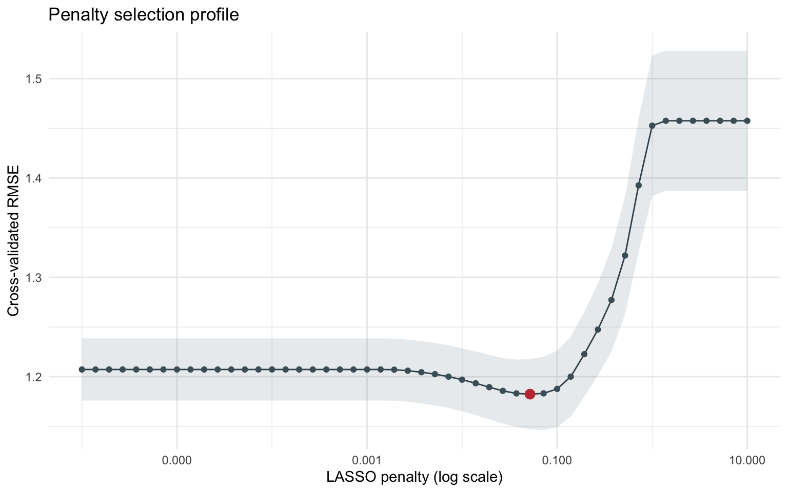
How λ is chosen
Because the number of variables in the final model depends on λ, we cannot set it arbitrarily. Instead, we use cross-validation:
Split the dataset into folds.
Fit the model across a grid of possible λ values.
Evaluate prediction accuracy (e.g., using root mean square error).
Select the λ that gives the best performance on unseen folds.
The final model is then re-fit using this optimal λ. At that penalty level, only the predictors with non-zero coefficients remain active.
Why this matters for our analysis
Our dataset is small but has many potential predictors. Using all of them risks overfitting.
Lasso automatically identifies which variables contribute most reliably to predicting violent intent.
The result is a compact set of predictors that balances parsimony (few variables) with accuracy (good predictions).
Data preparation
Code
load("../data/wrangled_data/dt_ana_base_jih.RData")criminal_raw <- dt_ana_base_jih %>%clean_names() %>%mutate(past_activism =ifelse(is.nan(past_activism), NA_real_, past_activism),across(where(is.factor), as.character) )criminal_df <- criminal_raw %>%select(-response_id,-gender, # all men-education,-religion, # all muslim-country,-peaceful_intent, # alternative DV-radical_attitudes, # too close to main DV-activist_intent, # fully missing in this sample-intuition, # fully missing in this sample-logic # fully missing in this sample ) %>%mutate(across(everything(), as.numeric)) %>%select(where(~!all(is.na(.)))) %>%drop_na(violent_intent)n_cases <-nrow(criminal_df)n_predictors <-ncol(criminal_df) -1list(observations = n_cases,predictors = n_predictors)
$observations
[1] 80

$predictors
[1] 14
The cleaned data contain 80 observations with 14 candidate predictors for violent intent. Despite the small sample, there is still a rich set of attitudinal and emotional measures to explore.
Variables such as collective relative deprivation and identity fusion still exhibit gaps, but median imputation (embedded in the modeling recipe below) keeps them in play without discarding cases.
Distributions and descriptive statistics
Code
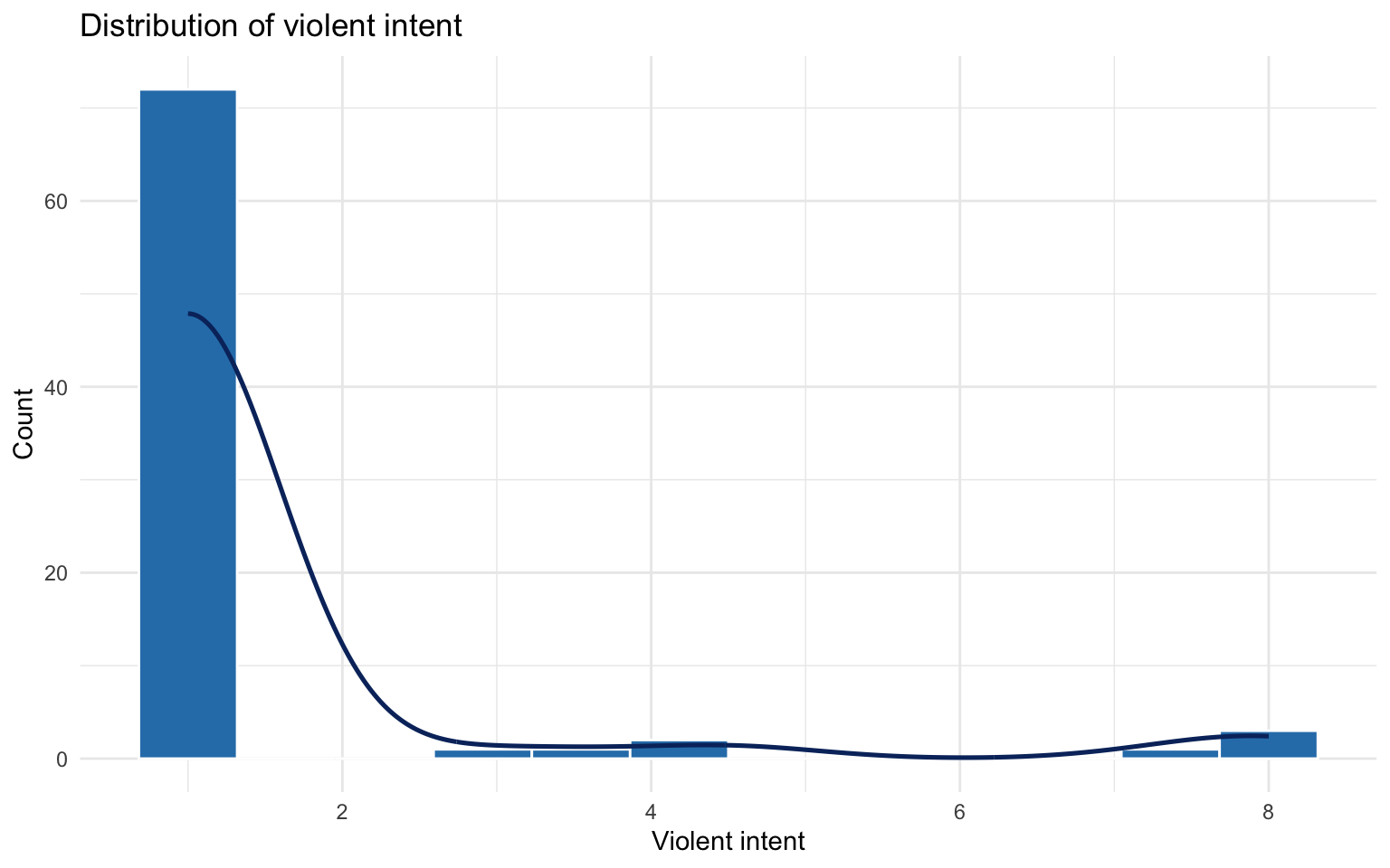
stat_df <- criminal_df %>%mutate(across(everything(), ~ifelse(is.na(.), median(., na.rm =TRUE), .)))p_vi <-ggplot(stat_df, aes(x = violent_intent)) +geom_histogram(bins =12, fill ="#2c7fb8", colour ="white") +geom_density(aes(y =after_stat(count)), colour ="#08306b", linewidth =0.9, alpha =0.4) +labs(x ="Violent intent", y ="Count", title ="Distribution of violent intent") +theme_minimal()p_vi
Violent intent is markedly skewed to the floor with a long tail at the high end, underscoring why regularization is critical: only a handful of detainees report elevated willingness to use violence.
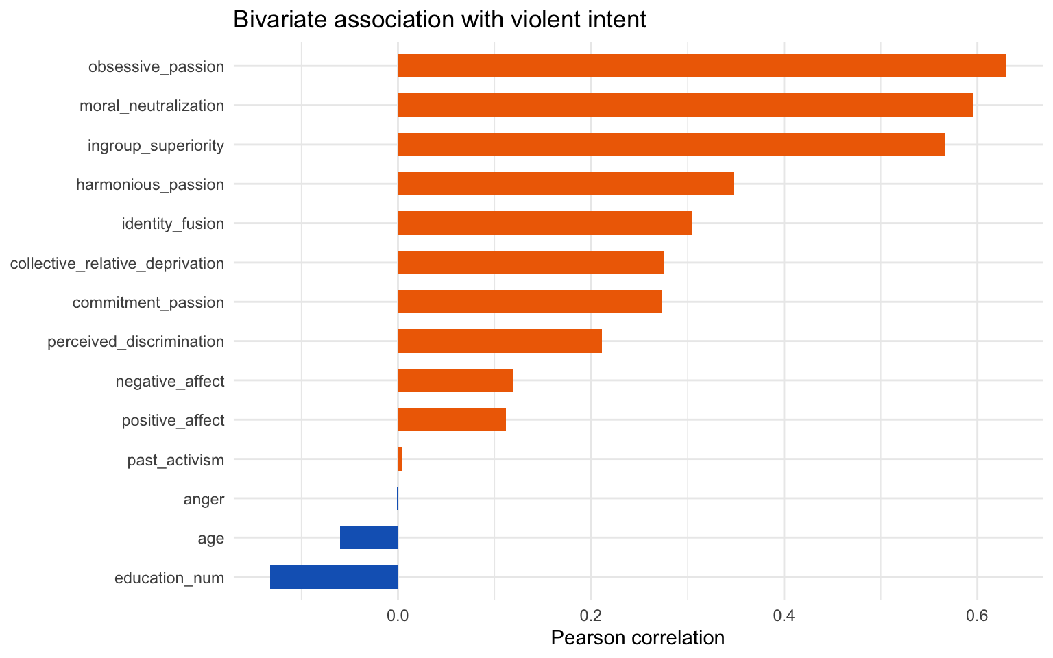
cor_summary <- stat_df %>%relocate(violent_intent) %>%summarise(across(-violent_intent, ~cor(.x, violent_intent))) %>%pivot_longer(everything(), names_to ="variable", values_to ="correlation") %>%mutate(variable =fct_reorder(variable, correlation))cor_summary %>%ggplot(aes(x = correlation, y = variable, fill = correlation >0)) +geom_col(width =0.6) +scale_fill_manual(values =c("TRUE"="#ef6c00", "FALSE"="#1565c0"), guide ="none") +labs(x ="Pearson correlation", y =NULL, title ="Bivariate association with violent intent") +theme_minimal()
Activist passion measures, perceived discrimination, and ingroup superiority already show positive simple correlations with violent intent, but multicollinearity and noise require a penalised model to adjudicate which survive joint estimation.
Modeling strategy
We adopt a tidy modeling workflow with five-fold cross-validation repeated 20 times (100 resamples total) to stabilise the penalty search. Predictors are median-imputed and standardized within each resample so that the LASSO penalty treats them on a comparable scale.
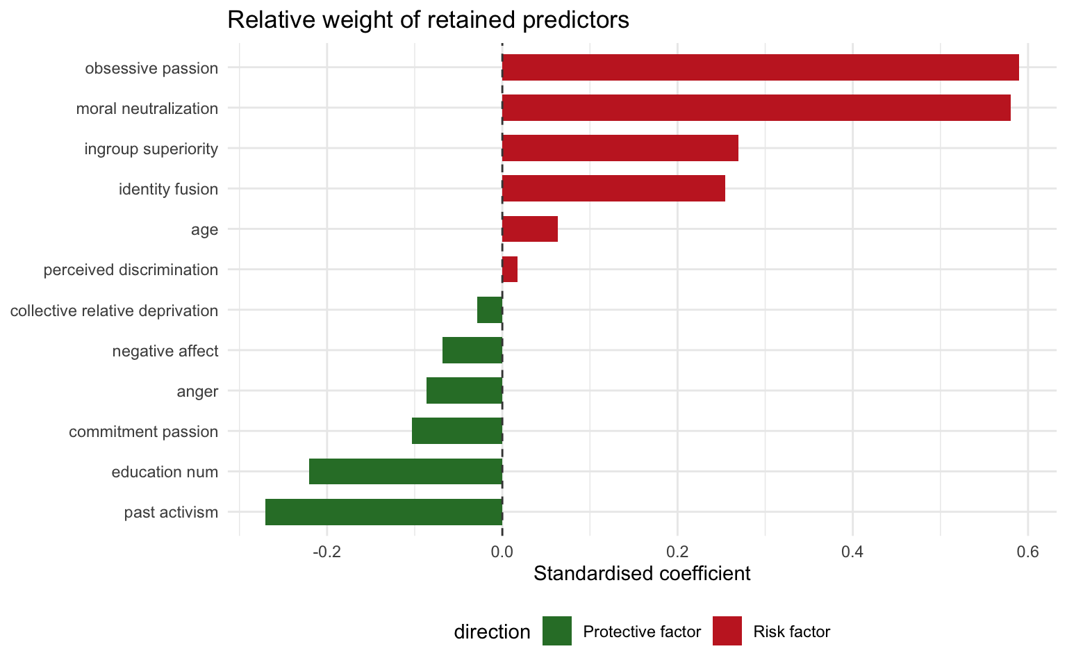
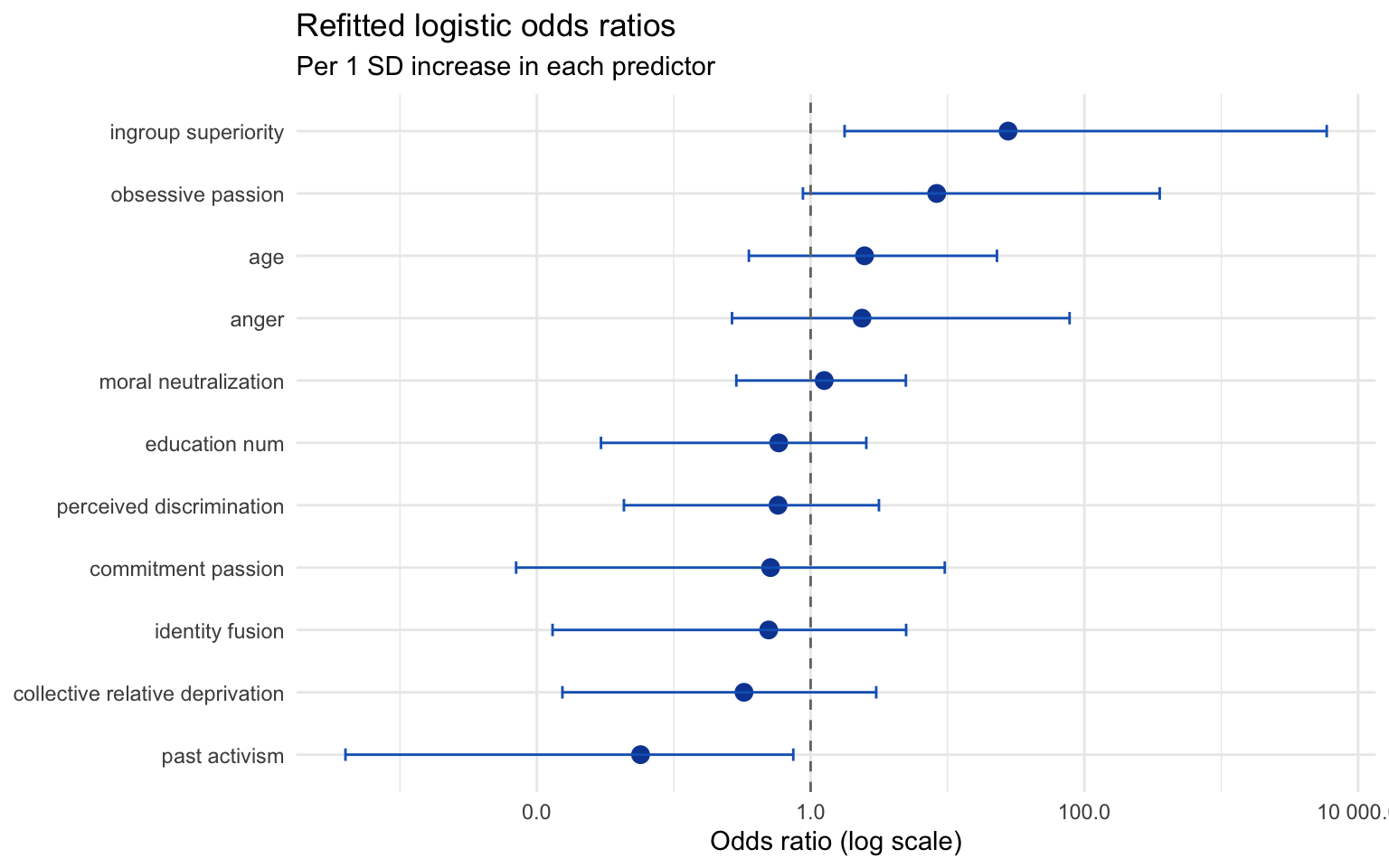
The coefficients represent the effect of a one standard deviation change in each predictor after median imputation. Positive estimates correspond to elevated violent intent, whereas negative values indicate attenuation.
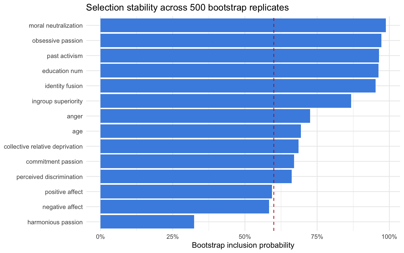
Variables with inclusion probability above the dashed line remain active in most bootstrap fits. Robust signals include moral neutralization (99%), obsessive passion (97%), past activism (96%), education num (96%), identity fusion (95%), ingroup superiority (87%), anger (73%), age (69%), collective relative deprivation (69%), commitment passion (67%), perceived discrimination (66%).
Effect sizes from the final logistic refit
To translate the sparse LASSO solution into interpretable quantities, violent intent scores above the floor category are treated as an “elevated” outcome. The selected predictors are median-imputed, standardised to one standard deviation, and refit with a plain logistic regression so that each coefficient reflects a 1 SD shift in its source variable.
8 of 80 detainees (10.0%) exhibit elevated violent intent, so the odds ratios still carry considerable uncertainty despite the simplified refit.
ingroup superiority remains the sharpest risk signal with an odds ratio of 27.71, whereas past activism leans protective (OR = 0.06).
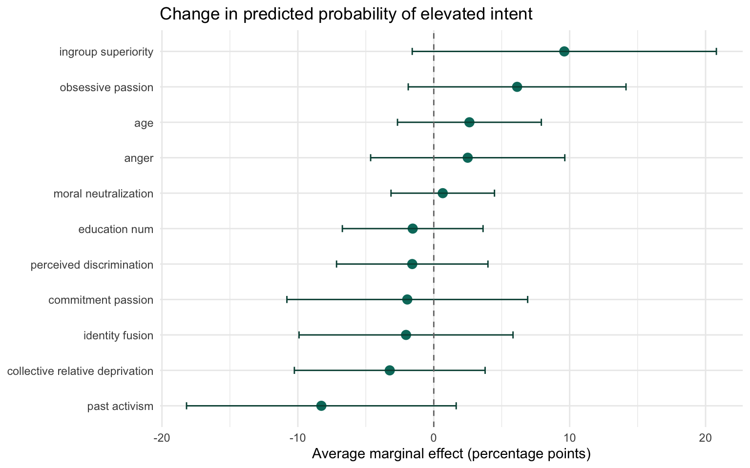
Average marginal effects translate these shifts into roughly 9.6 percentage points of additional risk for a 1 SD increase in ingroup superiority, contrasted with a -8.3 pp dip for past activism.
Code
effect_summary %>%arrange(desc(odds_ratio)) %>%mutate(`Odds ratio (95% CI)`=str_c(number(odds_ratio, accuracy =0.01),' (',number(or_low, accuracy =0.01),' – ',number(or_high, accuracy =0.01),')' ),`AME (pp, 95% CI)`=str_c(number(ame_pp, accuracy =0.1),' (',number(ame_low, accuracy =0.1),' – ',number(ame_high, accuracy =0.1),')' ),`p-value`=pvalue(p_value, accuracy =0.001) ) %>%select(Predictor = term_label,`Odds ratio (95% CI)`,`AME (pp, 95% CI)`,`p-value` ) %>%gt() %>%fmt_missing(columns =everything(), missing_text ='—') %>%tab_source_note(source_note = gt::md('Predictors are scaled to one standard deviation after median imputation. AME expresses the average percentage-point change in the probability of elevated intent.'))
Predictor
Odds ratio (95% CI)
AME (pp, 95% CI)
p-value
ingroup superiority
27.71 (1.77 – 5 892.84)
9.6 (-1.6 – 20.8)
0.073
obsessive passion
8.34 (0.88 – 355.11)
6.1 (-1.9 – 14.1)
0.129
age
2.48 (0.35 – 22.97)
2.6 (-2.7 – 7.9)
0.333
anger
2.37 (0.27 – 77.96)
2.5 (-4.6 – 9.6)
0.479
moral neutralization
1.26 (0.29 – 4.96)
0.7 (-3.1 – 4.5)
0.736
education num
0.59 (0.03 – 2.55)
-1.5 (-6.7 – 3.6)
0.556
perceived discrimination
0.58 (0.04 – 3.16)
-1.6 (-7.2 – 4.0)
0.579
commitment passion
0.51 (0.01 – 9.55)
-1.9 (-10.8 – 6.9)
0.666
identity fusion
0.49 (0.01 – 4.99)
-2.0 (-9.9 – 5.8)
0.604
collective relative deprivation
0.33 (0.02 – 3.01)
-3.2 (-10.3 – 3.8)
0.358
past activism
0.06 (0.00 – 0.75)
-8.3 (-18.2 – 1.6)
0.088
Predictors are scaled to one standard deviation after median imputation. AME expresses the average percentage-point change in the probability of elevated intent.
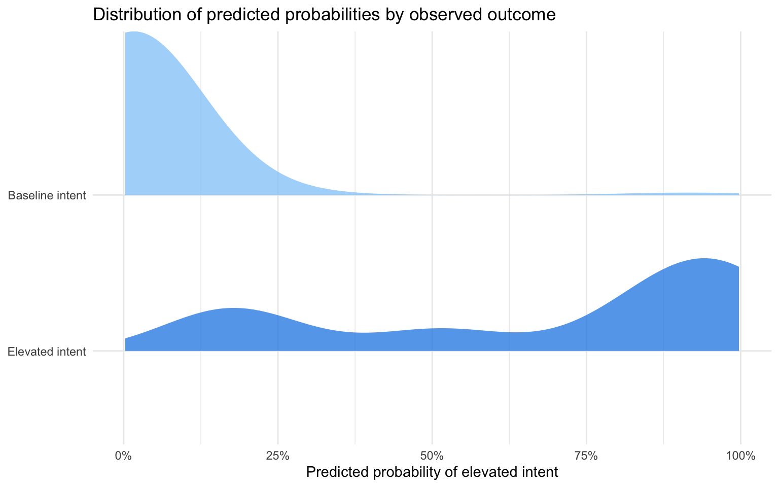
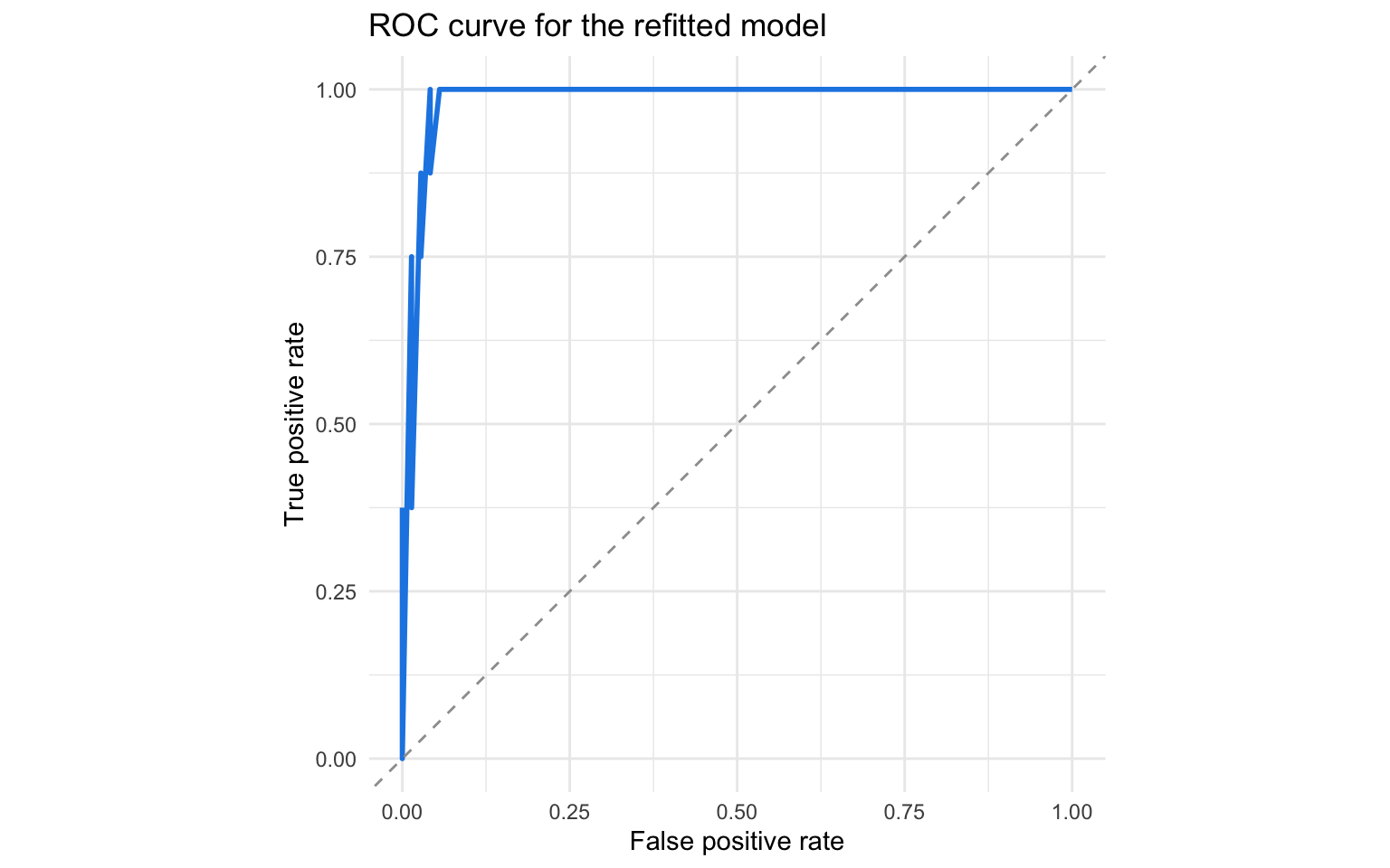
The refitted logistic attains an apparent AUC of 0.99 with a Brier score of 0.033. These values reflect in-sample performance; cross-validated optimism is already controlled upstream by the LASSO selection.
Code
prediction_df %>%mutate(truth =fct_relevel(truth, 'Elevated intent')) %>%ggplot(aes(x = .pred, y = truth, fill = truth)) +geom_density_ridges(alpha =0.75, colour =NA, scale =1.05) +scale_x_continuous(labels =percent_format(accuracy =1), limits =c(0, 1)) +scale_fill_manual(values =c('Baseline intent'='#90caf9', 'Elevated intent'='#1e88e5')) +guides(fill ='none') +labs(x ='Predicted probability of elevated intent',y =NULL,title ='Distribution of predicted probabilities by observed outcome' ) +theme_minimal()
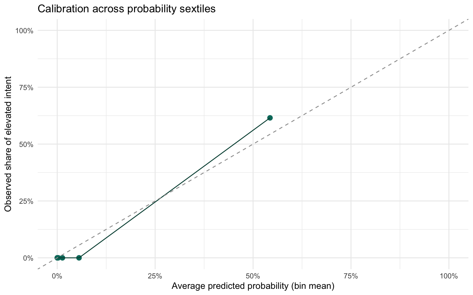
calibration_df %>%ggplot(aes(x = mean_pred, y = emp_rate)) +geom_point(size =2.5, colour ='#00796b') +geom_line(colour ='#004d40') +geom_abline(slope =1, intercept =0, linetype ='dashed', colour ='#9e9e9e') +scale_x_continuous(labels =percent_format(accuracy =1), limits =c(0, 1)) +scale_y_continuous(labels =percent_format(accuracy =1), limits =c(0, 1)) +labs(x ='Average predicted probability (bin mean)',y ='Observed share of elevated intent',title ='Calibration across probability sextiles' ) +theme_minimal()
The probability densities show clear separation between detainees with elevated intent and those at baseline, though the positive class remains extremely sparse. Calibration stays close to the diagonal for low-risk bins and becomes volatile once predictions exceed 20%, mirroring the limited number of elevated cases.
Interpretation and implications
Dominant risk marker: ingroup superiority increases the odds of elevated violent intent roughly 27.71-fold, corresponding to an average lift of 9.6 percentage points for a one SD increase.
Protective tendency: past activism delivers the largest downward shift (-8.3 pp) and an odds ratio below one, signaling a potential buffer against violent intent.
Practical takeaway: Even with shrinkage and a pared-down refit, only 8 detainees display elevated intent; any intervention should focus on consolidating the high-risk attitudinal profile while acknowledging the wide bands around point estimates.
Limitations
Small event count: Logistic coefficients are estimated from 8 elevated cases, so confidence intervals remain broad and sensitive to single observations.
Standardised interpretation: Odds ratios describe a one SD increase after median imputation; translating back to raw scale requires domain-specific knowledge of each measure.
In-sample evaluation: Performance diagnostics are apparent measures; external validation or temporal splits would be required to confirm transportability beyond this cohort.