3. Main Analyses Country Comparison

Load Data

Code

# load data for analysis
load("../data/wrangled_data/dt_ana_full.RData")

Analysis Strategy

We evaluate whether the predictive structure for violent intent differs across samples (countries; with a focal interest in the Jihadist sample) using two complementary strategies:

a multilevel model that separates within- from between-country effects and, in a second step, allows country-specific slopes;
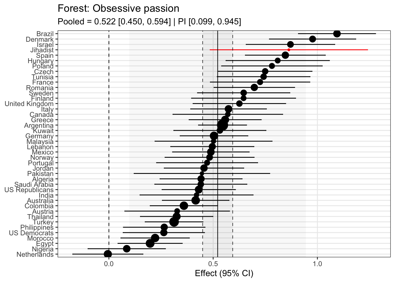
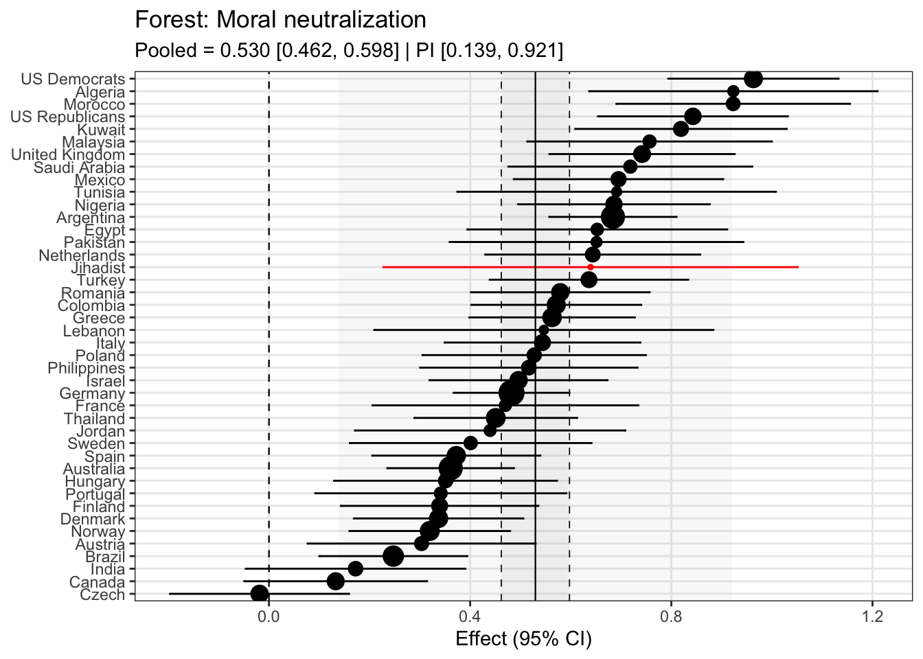
a two-step meta-analysis that fits the same model within each country, then pools coefficient estimates and tests heterogeneity.

Why both?

The multilevel model performs one-step partial pooling (stabilizing noisy country estimates via shrinkage), while the meta-analysis gives two-step, fully transparent country-by-country estimates with classic heterogeneity statistics (Q, τ², I²). Agreement between the two strengthens credibility.

Prepare Data

We use group-mean centering (suffix _cw) for individual-level predictors to estimate within-country relationships, and include country means (grand-mean centered) to estimate between-country differences. This avoids conflating contextual differences with individual-level effects.

Code

ana_df <- dt_ana_full %>%
  mutate(
    obsessive_passion_country_mean_c       = obsessive_passion_country_mean       - mean(obsessive_passion_country_mean,       na.rm = TRUE),
    moral_neutralization_country_mean_c    = moral_neutralization_country_mean    - mean(moral_neutralization_country_mean,    na.rm = TRUE),
    perceived_discrimination_country_mean_c= perceived_discrimination_country_mean- mean(perceived_discrimination_country_mean,na.rm = TRUE)
  )

Multilevel Models

Random Intercept Model

This model allows country-specific baselines for violent intent while estimating common within-country slopes for the centered predictors and between-country effects for country means.

Code

mod_ml_ri <- lmer(
  violent_intent ~
    obsessive_passion_cw +
    moral_neutralization_cw +
    perceived_discrimination_cw +
    obsessive_passion_country_mean_c +
    moral_neutralization_country_mean_c +
    perceived_discrimination_country_mean_c +
    (1 | country),
  data = ana_df, REML = TRUE
)

summ(mod_ml_ri)

Observations	10395
Dependent variable	violent_intent
Type	Mixed effects linear regression

AIC	33932.29
BIC	33997.53
Pseudo-R² (fixed effects)	0.48
Pseudo-R² (total)	0.50

Fixed Effects
	Est.	S.E.	t val.	d.f.	p
(Intercept)	2.13	0.04	55.44	38.15	0.00
obsessive_passion_cw	0.30	0.01	31.83	10350.23	0.00
moral_neutralization_cw	0.48	0.01	36.75	10350.23	0.00
perceived_discrimination_cw	0.28	0.01	22.76	10350.26	0.00
obsessive_passion_country_mean_c	0.25	0.06	4.13	38.16	0.00
moral_neutralization_country_mean_c	0.76	0.14	5.34	41.08	0.00
perceived_discrimination_country_mean_c	-0.15	0.12	-1.28	43.27	0.21
p values calculated using Satterthwaite d.f.

Random Effects
Group	Parameter	Std. Dev.
country	(Intercept)	0.24
Residual		1.23

Grouping Variables
Group	# groups	ICC
country	42	0.04

Code

# apa_lmer_summary(mod_ml_ri)

Random Slopes Model

We now allow country-specific slopes for the individual-level predictors. This addresses the question: do predictors of violent intent vary across samples? If so, we should see non-zero variance in the random slopes and improved model fit.

Code

mod_ml_rs <- lmer(
  violent_intent ~
    obsessive_passion_cw +
    moral_neutralization_cw +
    perceived_discrimination_cw +
    obsessive_passion_country_mean_c +
    moral_neutralization_country_mean_c +
    perceived_discrimination_country_mean_c +
    (1 +
       obsessive_passion_cw +
       moral_neutralization_cw +
       perceived_discrimination_cw | country),
  data = ana_df, REML = TRUE,
  control = lmerControl(optimizer = "bobyqa",
                        optCtrl = list(maxfun = 1e6))
)

summ(mod_ml_rs)

Observations	10395
Dependent variable	violent_intent
Type	Mixed effects linear regression

AIC	33626.69
BIC	33757.17
Pseudo-R² (fixed effects)	0.47
Pseudo-R² (total)	0.51

Fixed Effects
	Est.	S.E.	t val.	d.f.	p
(Intercept)	2.13	0.04	54.86	35.91	0.00
obsessive_passion_cw	0.31	0.02	14.42	41.33	0.00
moral_neutralization_cw	0.45	0.03	15.84	43.13	0.00
perceived_discrimination_cw	0.28	0.03	8.95	39.59	0.00
obsessive_passion_country_mean_c	0.32	0.05	6.08	39.15	0.00
moral_neutralization_country_mean_c	0.68	0.12	5.53	42.88	0.00
perceived_discrimination_country_mean_c	-0.17	0.10	-1.63	46.70	0.11
p values calculated using Satterthwaite d.f.

Random Effects
Group	Parameter	Std. Dev.
country	(Intercept)	0.24
country	obsessive_passion_cw	0.12
country	moral_neutralization_cw	0.16
country	perceived_discrimination_cw	0.18
Residual		1.20

Grouping Variables
Group	# groups	ICC
country	42	0.04

Code

mod_ml_ri_ml <- update(mod_ml_ri, REML = FALSE)
mod_ml_rs_ml <- update(mod_ml_rs, REML = FALSE)

model_comp <- anova(mod_ml_ri_ml, mod_ml_rs_ml)  # LRT for added random slopes

df_model_comp <- as.data.frame(model_comp)

df_model_comp %>% 
  kable(., caption = "Comparing fixed and random slope model") %>% 
  kable_styling(full_width = F, latex_options = c("hold_position", "scale-down"))

Comparing fixed and random slope model
	npar	AIC	BIC	logLik	-2*log(L)	Chisq	Df	Pr(>Chisq)
mod_ml_ri_ml	9	33896.46	33961.70	-16939.23	33878.46	NA	NA	NA
mod_ml_rs_ml	18	33594.34	33724.83	-16779.17	33558.34	320.1144	9	0

Model fit improves drasticially with random slopes (not suprisingly given the many different countries). We now assess how the Jihadist sample differs from the other samples.

Code

re_slopes <- broom.mixed::tidy(mod_ml_rs, effects = "ran_vals") %>%
  filter(grepl("_cw$", term)) %>% arrange(level, term) %>% 
  kable(., caption = "Random slopes of the multilevel model") %>% 
  kable_styling(full_width = F, latex_options = c("hold_position", "scale-down")) %>%
  scroll_box(width = "100%", height = "600px")

re_slopes

Random slopes of the multilevel model
effect	group	level	term	estimate	std.error
ran_vals	country	Algeria	moral_neutralization_cw	0.1920010	0.0803617
ran_vals	country	Algeria	obsessive_passion_cw	-0.0460439	0.0467942
ran_vals	country	Algeria	perceived_discrimination_cw	-0.0854935	0.0764843
ran_vals	country	Argentina	moral_neutralization_cw	0.1195694	0.0816873
ran_vals	country	Argentina	obsessive_passion_cw	-0.0084796	0.0588949
ran_vals	country	Argentina	perceived_discrimination_cw	-0.2774958	0.0561102
ran_vals	country	Australia	moral_neutralization_cw	-0.1265603	0.0722609
ran_vals	country	Australia	obsessive_passion_cw	-0.0364591	0.0592341
ran_vals	country	Australia	perceived_discrimination_cw	0.3136681	0.0883920
ran_vals	country	Austria	moral_neutralization_cw	-0.1398595	0.0706105
ran_vals	country	Austria	obsessive_passion_cw	-0.0587912	0.0527009
ran_vals	country	Austria	perceived_discrimination_cw	0.1518382	0.0828104
ran_vals	country	Brazil	moral_neutralization_cw	-0.1774514	0.0745897
ran_vals	country	Brazil	obsessive_passion_cw	0.2213237	0.0617989
ran_vals	country	Brazil	perceived_discrimination_cw	-0.1082629	0.0521255
ran_vals	country	Canada	moral_neutralization_cw	-0.2381855	0.0791714
ran_vals	country	Canada	obsessive_passion_cw	0.0339901	0.0716020
ran_vals	country	Canada	perceived_discrimination_cw	0.1450911	0.0902130
ran_vals	country	Colombia	moral_neutralization_cw	0.0245262	0.0801067
ran_vals	country	Colombia	obsessive_passion_cw	-0.0876488	0.0564467
ran_vals	country	Colombia	perceived_discrimination_cw	-0.0304747	0.0733970
ran_vals	country	Czech	moral_neutralization_cw	-0.3922567	0.0609153
ran_vals	country	Czech	obsessive_passion_cw	0.0906297	0.0525231
ran_vals	country	Czech	perceived_discrimination_cw	0.1737718	0.0660281
ran_vals	country	Denmark	moral_neutralization_cw	-0.1558344	0.0751766
ran_vals	country	Denmark	obsessive_passion_cw	0.1917418	0.0605169
ran_vals	country	Denmark	perceived_discrimination_cw	0.1809179	0.0819405
ran_vals	country	Egypt	moral_neutralization_cw	0.1596812	0.0843010
ran_vals	country	Egypt	obsessive_passion_cw	-0.1532270	0.0426987
ran_vals	country	Egypt	perceived_discrimination_cw	-0.2244731	0.0901010
ran_vals	country	Finland	moral_neutralization_cw	-0.1387134	0.0787455
ran_vals	country	Finland	obsessive_passion_cw	0.0754402	0.0637466
ran_vals	country	Finland	perceived_discrimination_cw	0.2154536	0.0943051
ran_vals	country	France	moral_neutralization_cw	-0.0610810	0.0847441
ran_vals	country	France	obsessive_passion_cw	0.0872091	0.0548869
ran_vals	country	France	perceived_discrimination_cw	0.0669262	0.1024786
ran_vals	country	Germany	moral_neutralization_cw	-0.0475450	0.0637135
ran_vals	country	Germany	obsessive_passion_cw	0.0180907	0.0568698
ran_vals	country	Germany	perceived_discrimination_cw	0.1504188	0.0707971
ran_vals	country	Greece	moral_neutralization_cw	0.0312585	0.0851622
ran_vals	country	Greece	obsessive_passion_cw	0.0160002	0.0639230
ran_vals	country	Greece	perceived_discrimination_cw	-0.1179148	0.0701434
ran_vals	country	Hungary	moral_neutralization_cw	-0.1113527	0.0664661
ran_vals	country	Hungary	obsessive_passion_cw	0.1633337	0.0517267
ran_vals	country	Hungary	perceived_discrimination_cw	-0.0847497	0.0646274
ran_vals	country	India	moral_neutralization_cw	-0.2505040	0.0609407
ran_vals	country	India	obsessive_passion_cw	-0.0136345	0.0513325
ran_vals	country	India	perceived_discrimination_cw	0.3003111	0.0737940
ran_vals	country	Israel	moral_neutralization_cw	-0.0325392	0.0738343
ran_vals	country	Israel	obsessive_passion_cw	0.1417073	0.0592403
ran_vals	country	Israel	perceived_discrimination_cw	-0.0128433	0.0702347
ran_vals	country	Italy	moral_neutralization_cw	-0.0090027	0.0765229
ran_vals	country	Italy	obsessive_passion_cw	0.0141864	0.0532230
ran_vals	country	Italy	perceived_discrimination_cw	-0.0211381	0.0717603
ran_vals	country	Jihadist	moral_neutralization_cw	0.0865049	0.1044518
ran_vals	country	Jihadist	obsessive_passion_cw	0.1244679	0.0778443
ran_vals	country	Jihadist	perceived_discrimination_cw	-0.2618898	0.0656130
ran_vals	country	Jordan	moral_neutralization_cw	0.0013468	0.0792926
ran_vals	country	Jordan	obsessive_passion_cw	-0.0089181	0.0455062
ran_vals	country	Jordan	perceived_discrimination_cw	-0.0771970	0.0791745
ran_vals	country	Kuwait	moral_neutralization_cw	0.1776016	0.0692008
ran_vals	country	Kuwait	obsessive_passion_cw	0.0108887	0.0492743
ran_vals	country	Kuwait	perceived_discrimination_cw	-0.0899695	0.0678726
ran_vals	country	Lebanon	moral_neutralization_cw	0.0701736	0.0925618
ran_vals	country	Lebanon	obsessive_passion_cw	0.0022176	0.0484758
ran_vals	country	Lebanon	perceived_discrimination_cw	-0.1644307	0.0879113
ran_vals	country	Malaysia	moral_neutralization_cw	0.1414571	0.0689734
ran_vals	country	Malaysia	obsessive_passion_cw	-0.0055680	0.0511423
ran_vals	country	Malaysia	perceived_discrimination_cw	-0.2912478	0.0843283
ran_vals	country	Mexico	moral_neutralization_cw	0.0701559	0.0837297
ran_vals	country	Mexico	obsessive_passion_cw	-0.0340595	0.0567684
ran_vals	country	Mexico	perceived_discrimination_cw	-0.0627637	0.0720584
ran_vals	country	Morocco	moral_neutralization_cw	0.2354822	0.0841350
ran_vals	country	Morocco	obsessive_passion_cw	-0.1518985	0.0459924
ran_vals	country	Morocco	perceived_discrimination_cw	-0.1159362	0.0875263
ran_vals	country	Netherlands	moral_neutralization_cw	0.0979797	0.0728834
ran_vals	country	Netherlands	obsessive_passion_cw	-0.2541074	0.0421493
ran_vals	country	Netherlands	perceived_discrimination_cw	0.3225652	0.0804401
ran_vals	country	Nigeria	moral_neutralization_cw	0.0975448	0.0698545
ran_vals	country	Nigeria	obsessive_passion_cw	-0.2381799	0.0490565
ran_vals	country	Nigeria	perceived_discrimination_cw	-0.0272519	0.0690244
ran_vals	country	Norway	moral_neutralization_cw	-0.1485635	0.0750772
ran_vals	country	Norway	obsessive_passion_cw	0.0199445	0.0633163
ran_vals	country	Norway	perceived_discrimination_cw	0.2352716	0.0900451
ran_vals	country	Pakistan	moral_neutralization_cw	0.0561238	0.0694043
ran_vals	country	Pakistan	obsessive_passion_cw	-0.0515232	0.0522035
ran_vals	country	Pakistan	perceived_discrimination_cw	0.0425067	0.0689245
ran_vals	country	Philippines	moral_neutralization_cw	-0.0202829	0.0716696
ran_vals	country	Philippines	obsessive_passion_cw	-0.1370612	0.0492047
ran_vals	country	Philippines	perceived_discrimination_cw	0.1025999	0.0668927
ran_vals	country	Poland	moral_neutralization_cw	-0.0038385	0.0702188
ran_vals	country	Poland	obsessive_passion_cw	0.1282037	0.0542743
ran_vals	country	Poland	perceived_discrimination_cw	-0.1193458	0.0619080
ran_vals	country	Portugal	moral_neutralization_cw	-0.0691270	0.0909377
ran_vals	country	Portugal	obsessive_passion_cw	-0.0160151	0.0641157
ran_vals	country	Portugal	perceived_discrimination_cw	-0.0475283	0.0897867
ran_vals	country	Romania	moral_neutralization_cw	0.0060282	0.0716728
ran_vals	country	Romania	obsessive_passion_cw	0.0680740	0.0547266
ran_vals	country	Romania	perceived_discrimination_cw	-0.0203428	0.0629523
ran_vals	country	Saudi Arabia	moral_neutralization_cw	0.1160802	0.0678950
ran_vals	country	Saudi Arabia	obsessive_passion_cw	-0.0388539	0.0439716
ran_vals	country	Saudi Arabia	perceived_discrimination_cw	-0.0196265	0.0680703
ran_vals	country	Spain	moral_neutralization_cw	-0.1171271	0.0725383
ran_vals	country	Spain	obsessive_passion_cw	0.1354121	0.0567547
ran_vals	country	Spain	perceived_discrimination_cw	-0.0387644	0.0708830
ran_vals	country	Sweden	moral_neutralization_cw	-0.0782831	0.0765485
ran_vals	country	Sweden	obsessive_passion_cw	0.0594792	0.0532810
ran_vals	country	Sweden	perceived_discrimination_cw	-0.0138309	0.0777131
ran_vals	country	Thailand	moral_neutralization_cw	-0.0842085	0.0609635
ran_vals	country	Thailand	obsessive_passion_cw	-0.1193783	0.0451944
ran_vals	country	Thailand	perceived_discrimination_cw	0.3394758	0.0633234
ran_vals	country	Tunisia	moral_neutralization_cw	0.0469952	0.0784233
ran_vals	country	Tunisia	obsessive_passion_cw	0.1141371	0.0437071
ran_vals	country	Tunisia	perceived_discrimination_cw	0.0018545	0.0783353
ran_vals	country	Turkey	moral_neutralization_cw	0.0901197	0.0698930
ran_vals	country	Turkey	obsessive_passion_cw	-0.1127295	0.0402284
ran_vals	country	Turkey	perceived_discrimination_cw	-0.1368012	0.0557231
ran_vals	country	US Democrats	moral_neutralization_cw	0.2834864	0.0644258
ran_vals	country	US Democrats	obsessive_passion_cw	-0.1298294	0.0503789
ran_vals	country	US Democrats	perceived_discrimination_cw	-0.0984404	0.0708602
ran_vals	country	US Republicans	moral_neutralization_cw	0.1845948	0.0743497
ran_vals	country	US Republicans	obsessive_passion_cw	-0.0405001	0.0492952
ran_vals	country	US Republicans	perceived_discrimination_cw	-0.0665710	0.0705959
ran_vals	country	United Kingdom	moral_neutralization_cw	0.1136054	0.0841577
ran_vals	country	United Kingdom	obsessive_passion_cw	0.0264287	0.0660298
ran_vals	country	United Kingdom	perceived_discrimination_cw	-0.1278869	0.0926761

Code

country_models <- ana_df %>%
  group_by(country) %>%
  do(model = lm(
    violent_intent ~
      obsessive_passion_gmz +
      moral_neutralization_gmz +
      perceived_discrimination_gmz,
    data = .
  ))

country_effects <- ana_df %>%
  group_by(country) %>%
  nest() %>%
  mutate(
    model = map(data, ~ lm(
      violent_intent ~
        obsessive_passion_gmz +
        moral_neutralization_gmz +
        perceived_discrimination_gmz,
      data = .x
    )),
    tidy = map(model, broom::tidy)
  ) %>%
  select(country, tidy) %>%
  unnest(tidy) %>%
  filter(term != "(Intercept)") %>%
  select(country, term, estimate, std.error)

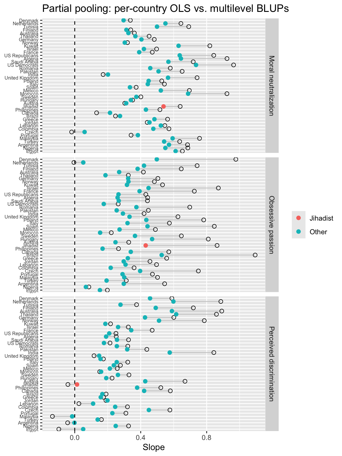
The following shrinkage (partial-pooling) contrasts, for each country and each predictor, the stand-alone country OLS (orinary least squares) slope with the multilevel Best Linear Unbiased Prediction (BLUP) slope which comes from the random-slopes model.

Hollow circle (OLS): the slope estimated by fitting a separate linear model within that country (no pooling).
Filled circle (BLUP): the country’s slope implied by the multilevel model = fixed effect + random deviation (i.e., after partial pooling).
Segment connecting them: the amount and direction of shrinkage from OLS → BLUP.
- Long segments = noisier country estimates (often small n) get pulled more toward the overall mean slope.
- Short segments = precise country estimates change little.

OLS

For each country, we fit a simple regression model just on that country’s data. The slope we get is the country-specific OLS slope.

Properties:

Uses only that country’s sample.
Very unbiased, but high variance if the country has a small sample size (noisy, unstable).

BLUB

The multilevel model’s estimate of a country’s slope = the global fixed slope plus that country’s random deviation.

Properties:

Shrinks noisy country slopes toward the overall mean slope (partial pooling).
Countries with large N or strong signal stay close to their OLS.
Countries with small N or noisy estimates get pulled toward the overall slope.

Code

# 3) Shrinkage plot: per-country OLS slopes vs. multilevel BLUPs (highlight Jihadist)
# Map *_gmz terms to *_cw to align labels
ols <- country_effects %>%
  dplyr::mutate(term = dplyr::recode(term,
    "obsessive_passion_gmz" = "obsessive_passion_cw",
    "moral_neutralization_gmz" = "moral_neutralization_cw",
    "perceived_discrimination_gmz" = "perceived_discrimination_cw"
  ))

# BLUP = fixed slope + random deviation
fixef_df <- broom.mixed::tidy(mod_ml_rs, effects = "fixed") %>%
  dplyr::filter(grepl("_cw$", term)) %>%
  dplyr::select(term, fix = estimate)

re_df <- broom.mixed::tidy(mod_ml_rs, effects = "ran_vals") %>%
  dplyr::filter(grepl("_cw$", term)) %>%
  dplyr::select(country = level, term, ran = estimate)

blup <- re_df %>% dplyr::left_join(fixef_df, by = "term") %>% dplyr::mutate(blup = fix + ran)

plot_df <- ols %>%
  dplyr::rename(ols = estimate) %>%
  dplyr::select(country, term, ols) %>%
  dplyr::inner_join(blup %>% dplyr::select(country, term, blup), by = c("country","term")) %>%
  dplyr::mutate(group = dplyr::if_else(country == "Jihadist", "Jihadist", "Other"),
                term_lab = dplyr::recode(term,
                  obsessive_passion_cw = "Obsessive passion",
                  moral_neutralization_cw = "Moral neutralization",
                  perceived_discrimination_cw = "Perceived discrimination"
                ))

ggplot(plot_df, aes(y = reorder(country, blup))) +
  geom_segment(aes(x = ols, xend = blup, yend = country), alpha = .5, color = "grey60") +
  geom_point(aes(x = ols), shape = 1, size = 2) +
  geom_point(aes(x = blup, color = group), size = 2) +
  geom_vline(xintercept = 0, linetype = 2) +
  facet_wrap(~term_lab, scales = "free_y", ncol = 1, strip.position = "right") +
  labs(
    x = "Slope", y = NULL, color = NULL,
    title = "Partial pooling: per-country OLS vs. multilevel BLUPs"
  ) +
  theme(
    axis.text.y = element_text(size = 6)  # smaller country labels
    # optional polish:
    # panel.spacing.y = unit(0.6, "lines")  # tighten vertical space between facets
  )

Two Step Meta-Analysis

To compare effects across countries transparently, we refitted the same country-level linear model using grand-mean standardized predictors (suffix _gmz), extracted per-country coefficients and standard errors. We now meta-analyze them with a random-effects model (REML). This yields an overall average effect and heterogeneity statistics (Q, τ², I²).

Code

meta_results <- country_effects %>%
  tidyr::nest(data = c(country, estimate, std.error)) %>%  # one row per term
  dplyr::mutate(
    .results = purrr::map(data, ~ metafor::rma(
      yi  = .x$estimate,
      sei = .x$std.error,
      method = "REML",
      slab = .x$country
    ))
  ) %>%
  dplyr::select(term, .results)

Code

# 4) Forest + Baujat (meta-analytic echo), adapted to generic slopes/SEs

# Helper: draw ggplot-style forest 
make_forest_generic <- function(rma_obj,
                                main_title = "Meta-analysis",
                                order_by = NULL,
                                show_prediction_interval = TRUE,
                                study_labels = NULL,
                                highlight = "Jihadist",          # <- NEW: what to highlight (character pattern(s) or logical vector)
                                highlight_color = "red") {       # <- NEW: highlight color
  # robust SE: prefer $sei if present, otherwise sqrt(vi)
  sei_vec <- if (length(rma_obj$sei) > 0) as.numeric(rma_obj$sei) else sqrt(as.numeric(rma_obj$vi))
  wi <- 1 / (sei_vec^2)

  slab_vec <- if (!is.null(study_labels)) study_labels else rma_obj$slab

  # build highlight flag (case-insensitive substring match OR logical vector)
  hl_flag <- rep(FALSE, length(slab_vec))
  if (is.logical(highlight) && length(highlight) == length(slab_vec)) {
    hl_flag <- highlight
  } else if (is.character(highlight) && length(highlight) > 0) {
    for (pat in highlight) hl_flag <- hl_flag | grepl(pat, slab_vec, ignore.case = TRUE)
  }

  df <- tibble(
    slab = slab_vec,
    yi   = as.numeric(rma_obj$yi),
    sei  = sei_vec,
    ci_l = yi - qnorm(.975) * sei_vec,
    ci_u = yi + qnorm(.975) * sei_vec,
    w    = wi,
    hl   = ifelse(hl_flag, "highlight", "other")
  )

  if (!is.null(order_by) && order_by %in% names(df)) {
    df <- arrange(df, .data[[order_by]])
  }

  # overall pooled effect (+ CI + optional PI)
  overall <- tibble(
    slab = "Overall (REML)",
    yi   = as.numeric(rma_obj$b),
    ci_l = as.numeric(rma_obj$ci.lb),
    ci_u = as.numeric(rma_obj$ci.ub)
  )

  # prediction interval if available
  pi_band <- NULL
  if (isTRUE(show_prediction_interval)) {
    pr <- tryCatch(predict(rma_obj, transf = NULL), error = function(e) NULL)
    if (!is.null(pr) && !any(is.na(c(pr$pi.lb, pr$pi.ub)))) {
      pi_band <- c(pr$pi.lb, pr$pi.ub)
    }
  }

  g <- ggplot(bind_rows(df %>% select(-w, -sei), overall),
              aes(x = yi, y = reorder(slab, yi))) +
    geom_vline(xintercept = 0, linetype = 2, linewidth = 0.4) +
    annotate("rect",
             xmin = overall$ci_l[1], xmax = overall$ci_u[1],
             ymin = -Inf, ymax = Inf,
             alpha = 0.06) +
    {if (!is.null(pi_band))
      annotate("rect",
               xmin = pi_band[1], xmax = pi_band[2],
               ymin = -Inf, ymax = Inf,
               alpha = 0.04)} +
    # Error bars + points ONLY for study rows, colored by highlight flag
    geom_errorbarh(data = df,
                   aes(xmin = ci_l, xmax = ci_u, color = hl),
                   height = .15) +
    geom_point(data = df,
               aes(color = hl, size = pmin(w / max(w, na.rm = TRUE), 1)),
               show.legend = FALSE) +
    # pooled vertical + CI
    geom_vline(xintercept = overall$yi[1], linewidth = 0.4) +
    geom_vline(xintercept = overall$ci_l[1], linetype = "dashed", linewidth = 0.3) +
    geom_vline(xintercept = overall$ci_u[1], linetype = "dashed", linewidth = 0.3) +
    scale_color_manual(values = c(other = "black", highlight = highlight_color), guide = "none") +
    labs(x = "Effect (95% CI)",
         y = NULL,
         title = main_title,
         subtitle = paste0(
           "Pooled = ",
           formatC(overall$yi[1], digits = 3, format = "f"),
           " [", formatC(overall$ci_l[1], digits = 3, format = "f"),
           ", ", formatC(overall$ci_u[1], digits = 3, format = "f"), "]",
           if (!is.null(pi_band)) paste0(
             " | PI [",
             formatC(pi_band[1], digits = 3, format = "f"), ", ",
             formatC(pi_band[2], digits = 3, format = "f"), "]"
           ) else ""
         )) +
    theme_bw() +
    theme(panel.grid.minor = element_blank())

  return(g)
}

# Helper: draw funnel (generic) with highlighting
make_funnel_generic <- function(rma_obj,
                                main_title = "Funnel plot",
                                refline = 0,
                                levels = c(90, 95, 99),
                                grayscale = c("white", "gray55", "gray75"),
                                legend_pos = "topright",
                                highlight = "Jihadist",         # <- NEW
                                highlight_color = "red") {       # <- NEW
  # Ensure we have yi/vi/sei
  yi <- as.numeric(rma_obj$yi)
  vi <- if (!is.null(rma_obj$vi)) as.numeric(rma_obj$vi) else (as.numeric(rma_obj$sei))^2
  sei <- sqrt(vi)

  slab_vec <- rma_obj$slab
  # highlight flag (same rules as forest)
  hl_flag <- rep(FALSE, length(slab_vec))
  if (is.logical(highlight) && length(highlight) == length(slab_vec)) {
    hl_flag <- highlight
  } else if (is.character(highlight) && length(highlight) > 0) {
    for (pat in highlight) hl_flag <- hl_flag | grepl(pat, slab_vec, ignore.case = TRUE)
  }

  # Trim-and-fill on the fitted model
  tf <- tryCatch(trimfill(rma_obj), error = function(e) rma_obj)

  # PET / PEESE regressions
  pet   <- tryCatch(rma(yi = yi, sei = sei, mods = ~ sei), error = function(e) NULL)
  peese <- tryCatch(rma(yi = yi, sei = sei, mods = ~ I(sei^2)), error = function(e) NULL)

  reml_b <- as.numeric(rma_obj$b)

  funnel(tf, level = levels, shade = grayscale, refline = refline,
         legend = legend_pos,
         main = paste0(
           main_title, "\n",
           "REML = ", formatC(reml_b, digits = 2, format = "f"),
           if (!is.null(pet))   paste0(",  PET = ",   formatC(pet$b[1],   digits = 2, format = "f")) else "",
           if (!is.null(peese)) paste0(",  PEESE = ", formatC(peese$b[1], digits = 2, format = "f")) else "",
           ",  n = ", length(yi)
         ))

  # pooled marker
  abline(v = reml_b, lty = "dashed")
  points(x = reml_b, y = 0, cex = 1.4, pch = 17)

  # PEESE curve + point
  if (!is.null(peese) && length(peese$b) >= 2) {
    sei_grid <- seq(0, max(sei, na.rm = TRUE), length.out = 1000)
    vi_grid  <- sei_grid^2
    yi_grid  <- as.numeric(peese$b[1]) + as.numeric(peese$b[2]) * vi_grid
    lines(x = yi_grid, y = sei_grid)
    points(x = as.numeric(peese$b[1]), y = 0, cex = 1.3, pch = 5)
  }

  # PET line + point + CI segment
  if (!is.null(pet) && length(pet$b) >= 2) {
    abline(a = -as.numeric(pet$b[1]) / as.numeric(pet$b[2]),
           b =  1 / as.numeric(pet$b[2]))
    points(x = as.numeric(pet$b[1]), y = 0, cex = 1.2)
    segments(x0 = as.numeric(pet$ci.lb[1]), y0 = 0,
             x1 = as.numeric(pet$ci.ub[1]), y1 = 0,
             lty = "dashed")
  }

  # OVERDRAW highlighted studies in red so they pop
  if (any(hl_flag, na.rm = TRUE)) {
    points(x = yi[hl_flag], y = sei[hl_flag], pch = 19, col = highlight_color, cex = 1.2)
  }

  invisible(list(trimfill = tf, PET = pet, PEESE = peese))
}

# Driver: pass highlight through
# Driver: iterate meta_results and produce Forest + Funnel with section headers
plot_meta_suite <- function(meta_results, add_funnel = TRUE,
                            highlight = "Jihadist", highlight_color = "red") {
  terms <- unique(meta_results$term)
  for (tm in terms) {
    mobj <- meta_results %>%
      filter(term == tm) %>%
      pull(.results) %>%
      .[[1]]

    pretty <- dplyr::recode(tm,
      "obsessive_passion_gmz"     = "Obsessive passion",
      "moral_neutralization_gmz"  = "Moral neutralization",
      "perceived_discrimination_gmz" = "Perceived discrimination",
      .default = tm
    )

    # Emit a second-level markdown header so Quarto renders it
    cat("\n\n## ", pretty, "\n\n")

    print(make_forest_generic(mobj,
                              main_title = paste0("Forest: ", pretty),
                              order_by = NULL,
                              show_prediction_interval = TRUE,
                              highlight = highlight,
                              highlight_color = highlight_color))

    if (add_funnel)
      make_funnel_generic(mobj,
                          main_title = paste0("Funnel: ", pretty),
                          highlight = highlight,
                          highlight_color = highlight_color)
  }
}

# Run the meta suite (set add_funnel = FALSE if you don’t want funnels)
plot_meta_suite(meta_results, add_funnel = TRUE)

Obsessive passion

Warning: `geom_errobarh()` was deprecated in ggplot2 4.0.0.
ℹ Please use the `orientation` argument of `geom_errorbar()` instead.

`height` was translated to `width`.

Moral neutralization

`height` was translated to `width`.

Perceived discrimination

`height` was translated to `width`.

Load Data

Analysis Strategy

Prepare Data

Multilevel Models

Random Intercept Model

Random Slopes Model

Two Step Meta-Analysis

Obsessive passion

Moral neutralization

Perceived discrimination

References