Alert - This a masked version for internal use only
3. Main Analyses Country Comparison
Load Data
Code
# load data for analysisload("../data/wrangled_data/dt_ana_full.RData")
Analysis Strategy
We evaluate whether the predictive structure for violent intent differs across samples (countries; with a focal interest in the Jihadist sample) using two complementary strategies:
a multilevel model that separates within- from between-country effects and, in a second step, allows country-specific slopes;
a two-step meta-analysis that fits the same model within each country, then pools coefficient estimates and tests heterogeneity.
Why both?
The multilevel model performs one-step partial pooling (stabilizing noisy country estimates via shrinkage), while the meta-analysis gives two-step, fully transparent country-by-country estimates with classic heterogeneity statistics (Q, τ², I²). Agreement between the two strengthens credibility.
Prepare Data
We use group-mean centering (suffix _cw) for individual-level predictors to estimate within-country relationships, and include country means (grand-mean centered) to estimate between-country differences. This avoids conflating contextual differences with individual-level effects.
This model allows country-specific baselines for violent intent while estimating common within-country slopes for the centered predictors and between-country effects for country means.
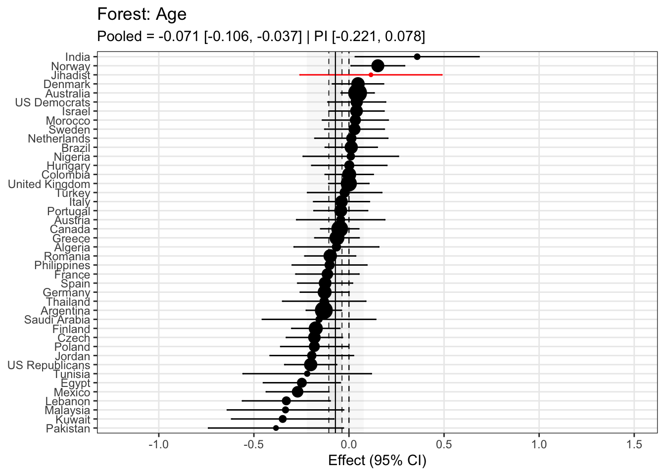
We now allow country-specific slopes for the individual-level predictors. This addresses the question: do predictors of violent intent vary across samples? If so, we should see non-zero variance in the random slopes and improved model fit.
model_comp <-anova(mod_ml_ri_ml, mod_ml_rs_ml) # LRT for added random slopesdf_model_comp <-as.data.frame(model_comp)df_model_comp %>%kable(., caption ="Comparing fixed and random slope model") %>%kable_styling(full_width = F, latex_options =c("hold_position", "scale-down"))
Comparing fixed and random slope model
npar
AIC
BIC
logLik
-2*log(L)
Chisq
Df
Pr(>Chisq)
mod_ml_ri_ml
35
33757.23
34010.94
-16843.61
33687.23
NA
NA
NA
mod_ml_rs_ml
44
33453.18
33772.14
-16682.59
33365.18
322.0501
9
0
Model fit improves drasticially with random slopes (not suprisingly given the many different countries). We now assess how the Jihadist sample differs from the other samples.
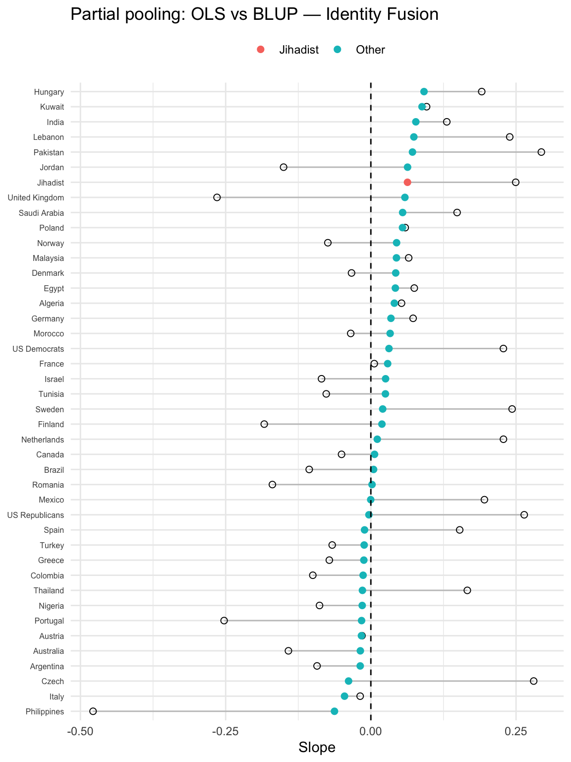
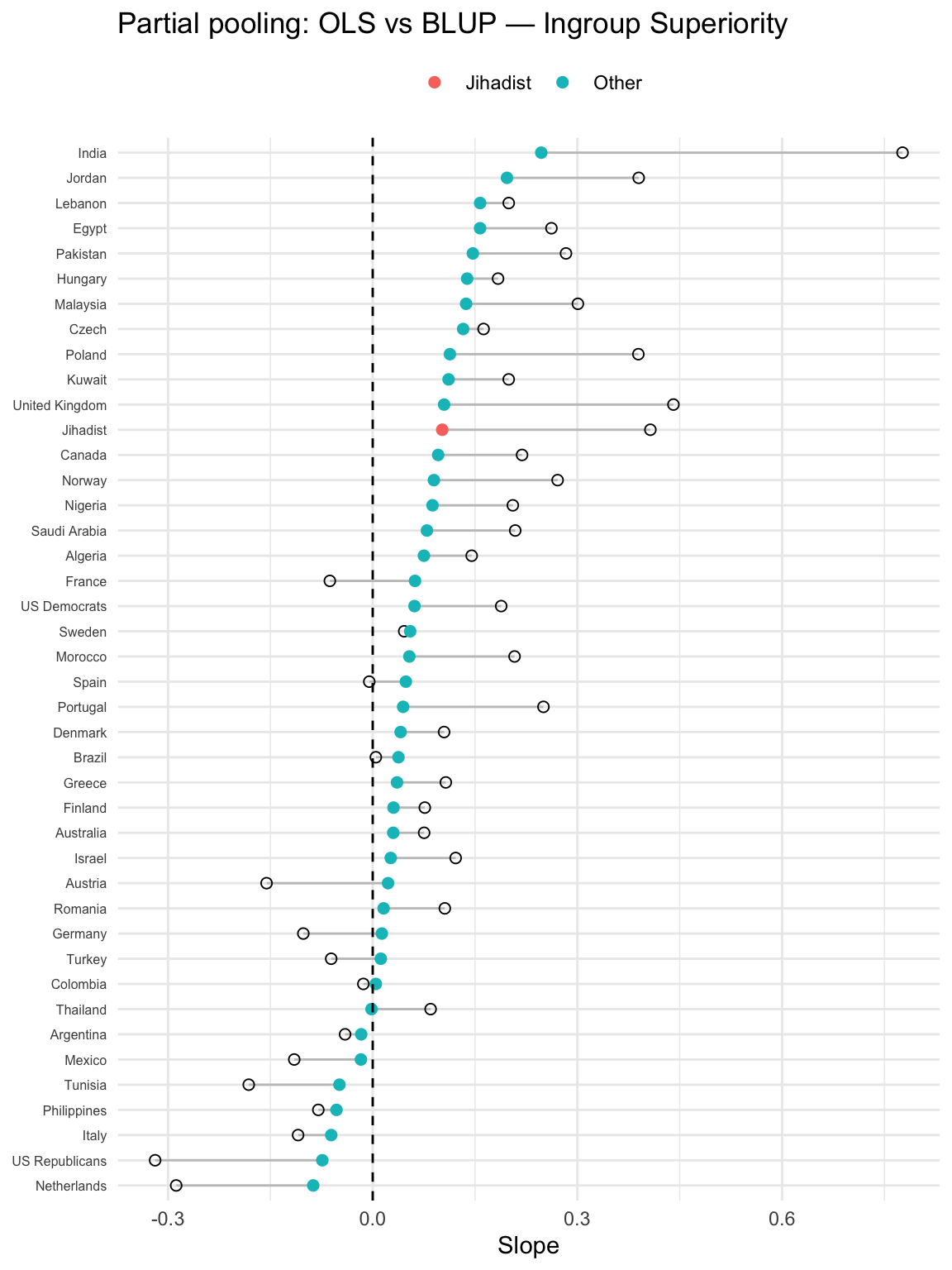
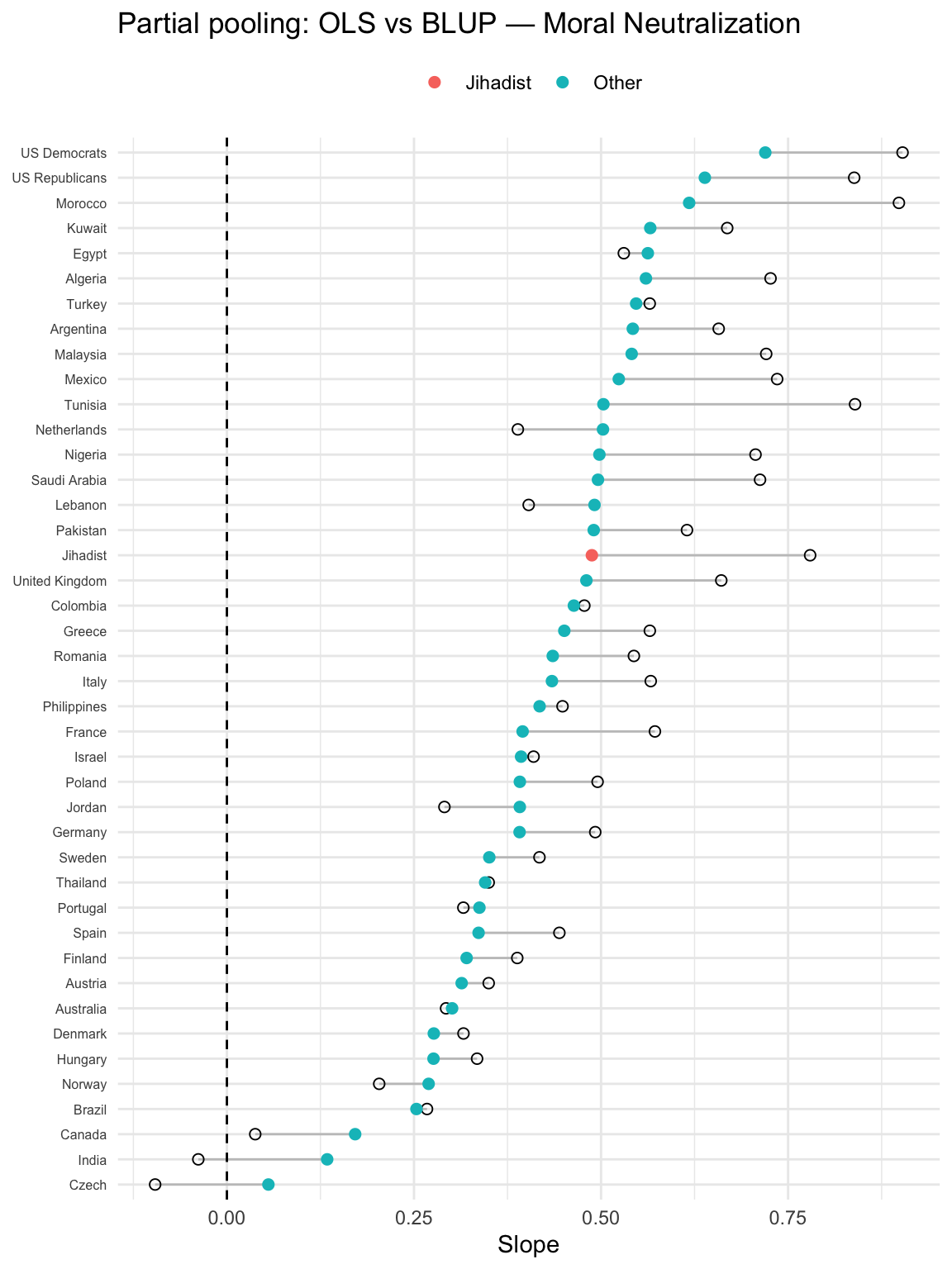
The following shrinkage (partial-pooling) contrasts, for each country and each predictor, the stand-alone country OLS (orinary least squares) slope with the multilevel Best Linear Unbiased Prediction (BLUP) slope which comes from the random-slopes model.
Hollow circle (OLS): the slope estimated by fitting a separate linear model within that country (no pooling).
Filled circle (BLUP): the country’s slope implied by the multilevel model = fixed effect + random deviation (i.e., after partial pooling).
Segment connecting them: the amount and direction of shrinkage from OLS → BLUP.
Long segments = noisier country estimates (often small n) get pulled more toward the overall mean slope.
Short segments = precise country estimates change little.
OLS
For each country, we fit a simple regression model just on that country’s data. The slope we get is the country-specific OLS slope.
Properties:
Uses only that country’s sample.
Very unbiased, but high variance if the country has a small sample size (noisy, unstable).
BLUB
The multilevel model’s estimate of a country’s slope = the global fixed slope plus that country’s random deviation.
Properties:
Shrinks noisy country slopes toward the overall mean slope (partial pooling).
Countries with large N or strong signal stay close to their OLS.
Countries with small N or noisy estimates get pulled toward the overall slope.
Code
# 3) Shrinkage plot: per-country OLS slopes vs. multilevel BLUPs (highlight Jihadist)# Map *_gmz terms to *_cw to align labels# 1) Recode gmz predictors to their CW counterparts (for easier matching)ols <- country_effects %>%mutate(term =str_replace(term, "_gmz$", "_cw"))# 2) Get fixed effects (all CW terms) from the random-slope modelfixef_df <- broom.mixed::tidy(mod_ml_rs, effects ="fixed") %>%filter(str_detect(term, "_cw$")) %>%select(term, fix = estimate)# 3) Get random deviations (all CW terms) per countryre_df <- broom.mixed::tidy(mod_ml_rs, effects ="ran_vals") %>%filter(str_detect(term, "_cw$")) %>%select(country = level, term, ran = estimate)# 4) Compute BLUPs = fixed slope + random deviationblup <- re_df %>%left_join(fixef_df, by ="term") %>%mutate(blup = fix + ran)# 5) Combine OLS and BLUPs into a single plotting datasetplot_df <- ols %>%rename(ols = estimate) %>%select(country, term, ols) %>%inner_join(blup %>%select(country, term, blup), by =c("country","term")) %>%mutate(group =if_else(country =="Jihadist", "Jihadist", "Other"),term_lab = term %>%str_remove("_cw$") %>%str_replace_all("_", " ") %>%str_to_title() # nice readable labels )# 6) Plot# Helper: one predictor's shrinkage plotshrinkage_plot_one <-function(df, term_label) { d <- df %>% dplyr::filter(term_lab == term_label)ggplot(d, aes(y = forcats::fct_reorder(country, blup))) +geom_segment(aes(x = ols, xend = blup, yend = country), alpha =0.5, color ="grey60") +geom_point(aes(x = ols), shape =1, size =2) +geom_point(aes(x = blup, color = group), size =2) +geom_vline(xintercept =0, linetype =2) +labs(x ="Slope",y =NULL,color =NULL,title =paste0("Partial pooling: OLS vs BLUP — ", term_label) ) +theme_minimal() +theme(axis.text.y =element_text(size =6),legend.position ="top" )}# Emit a single tabset with one tab per predictorrender_shrinkage_tabs <-function(df) { labs <-sort(unique(df$term_lab))# blank line before fenced div is IMPORTANTcat("\n\n::: {.panel-tabset}\n\n")for (lb in labs) {# each heading becomes a tab (no {.tabset} here)cat("\n")cat("#### ", lb, "\n\n", sep ="")print(shrinkage_plot_one(df, lb))cat("\n") }cat(":::\n")}# Render the tabsrender_shrinkage_tabs(plot_df)
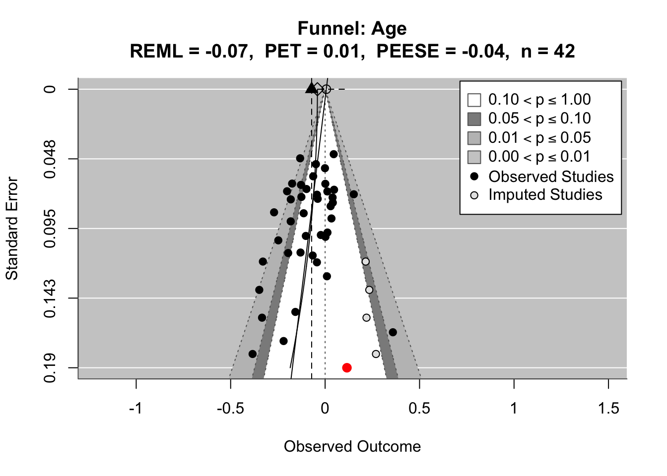
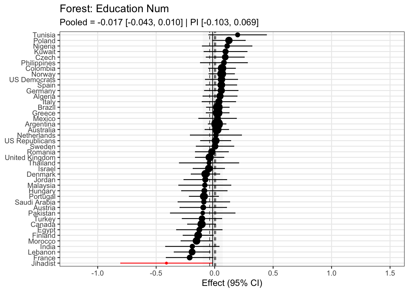
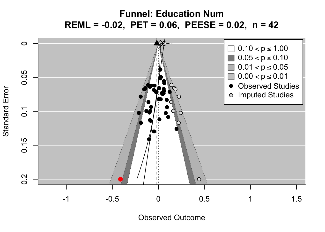
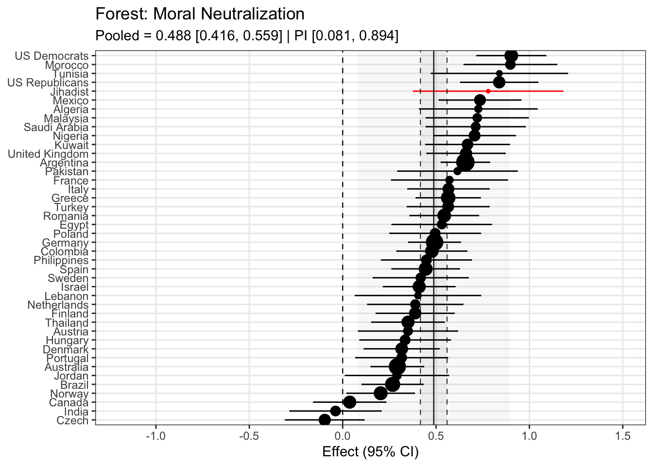
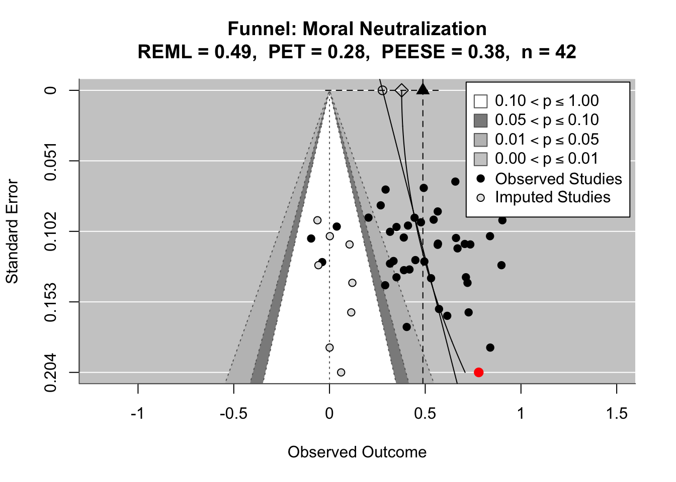
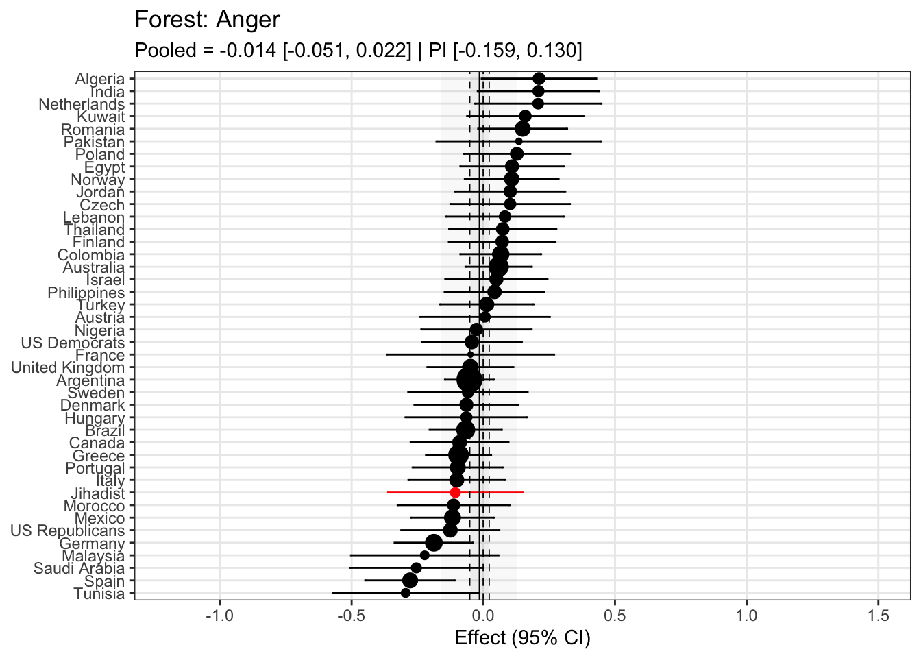
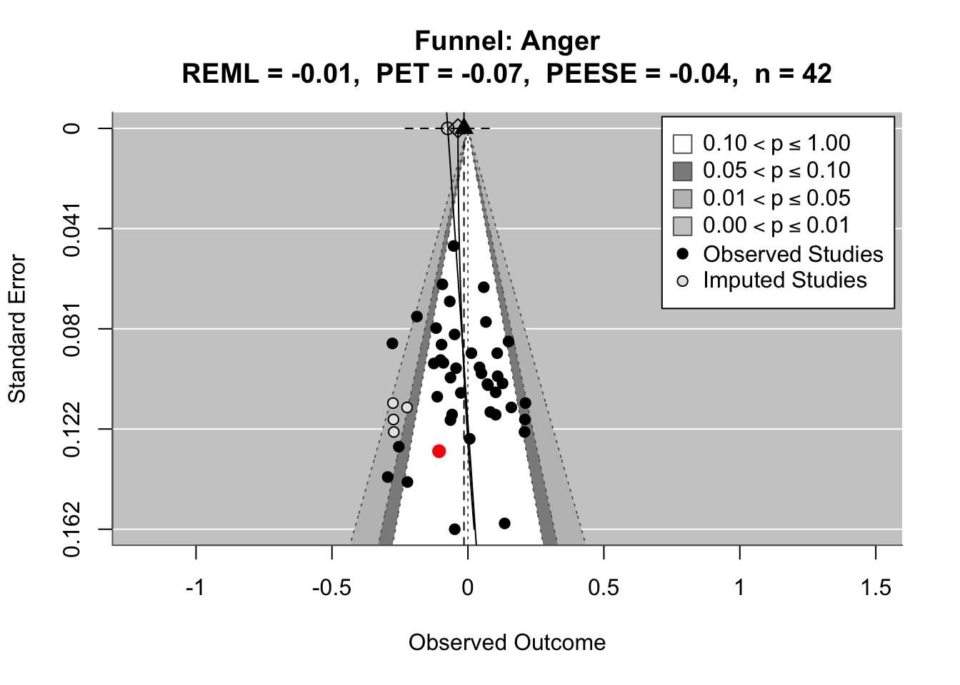
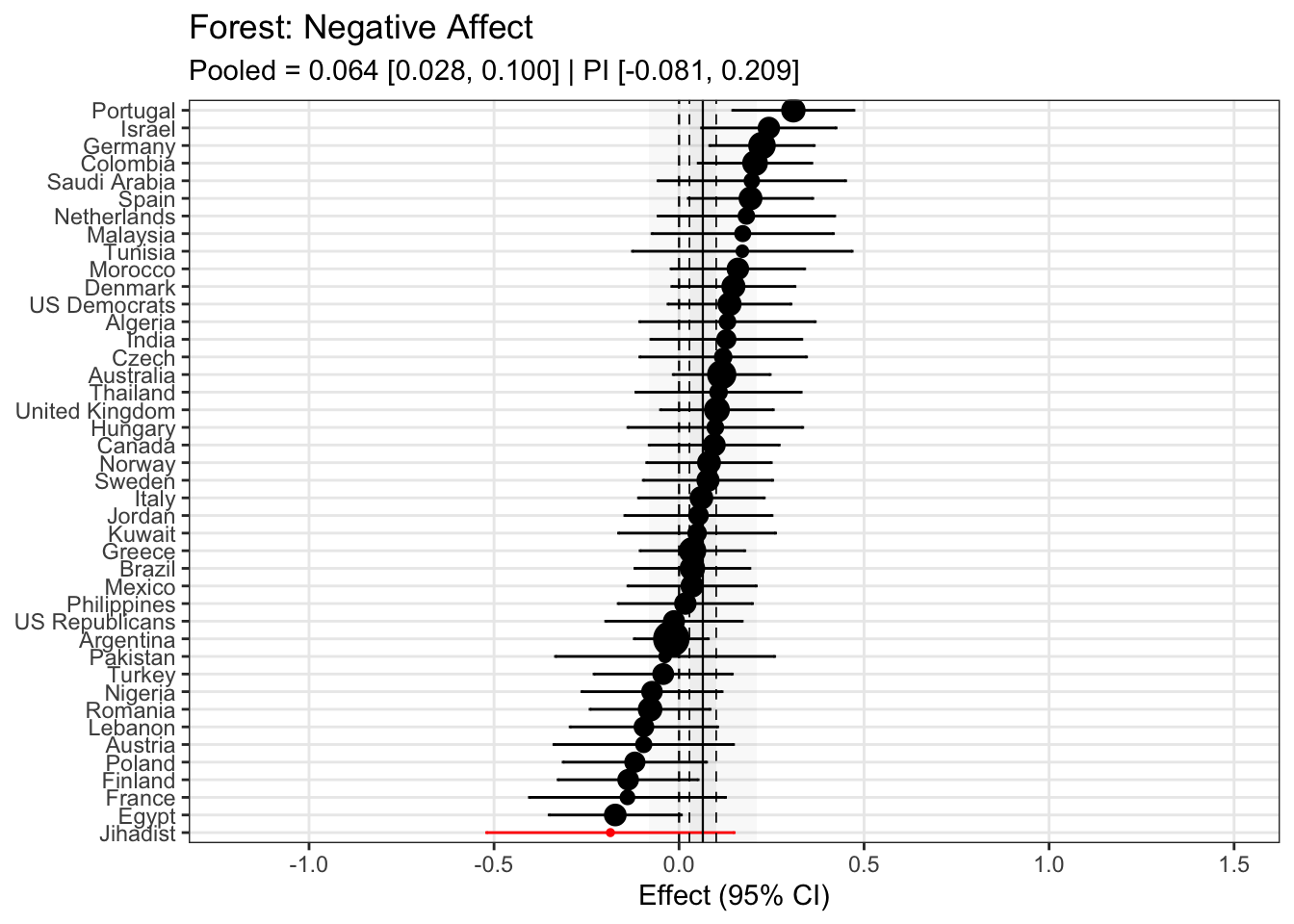
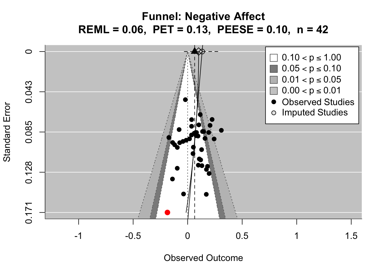
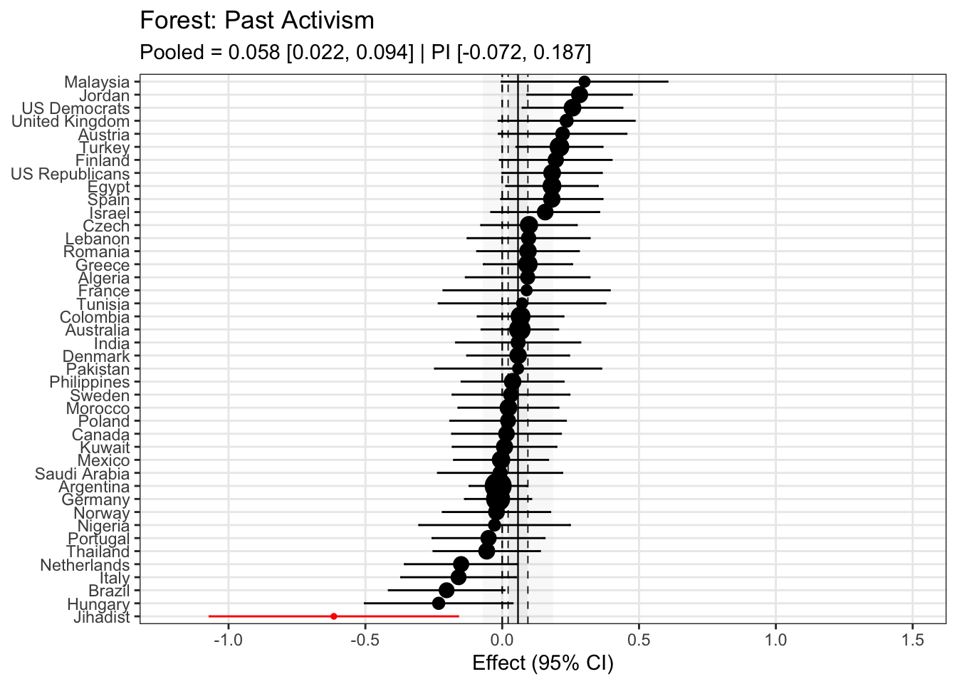
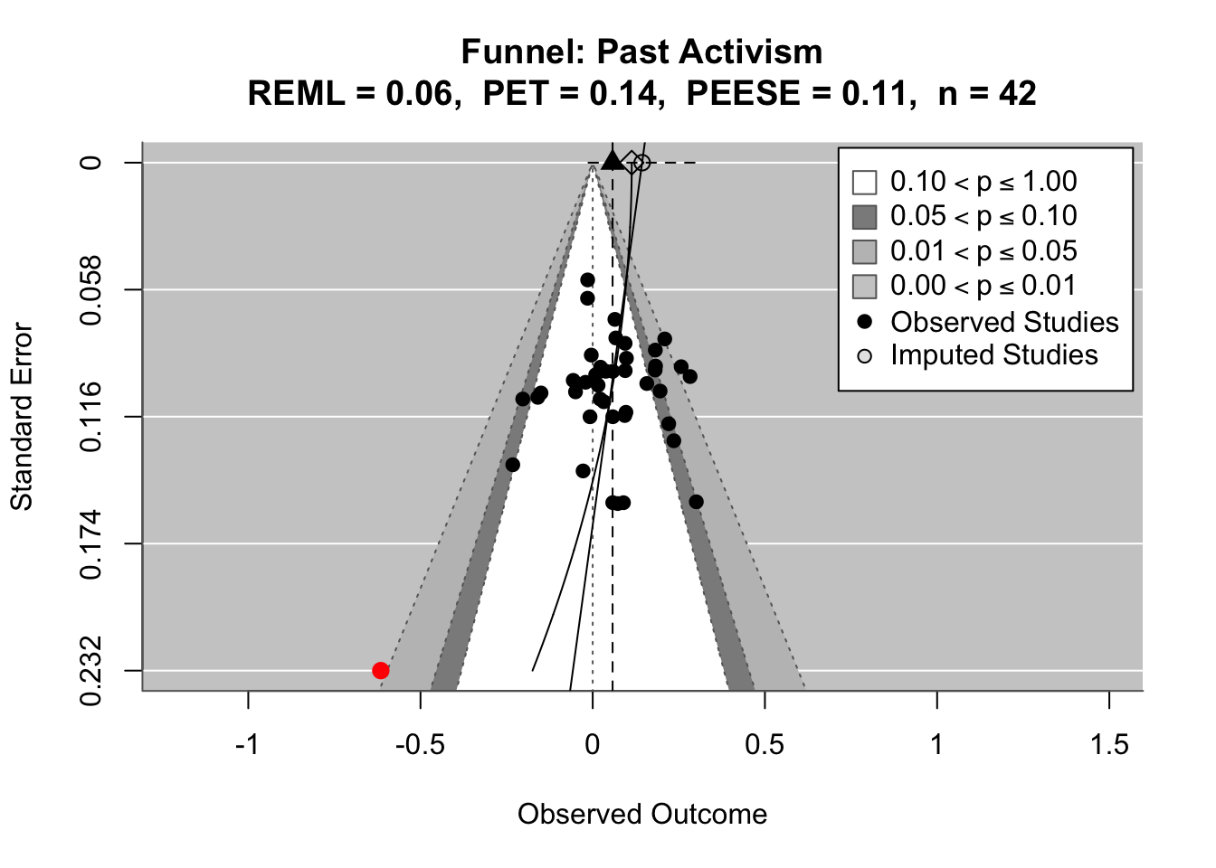
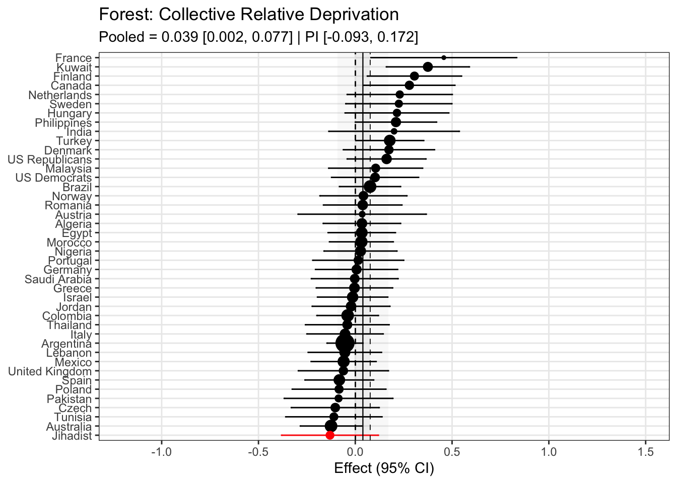
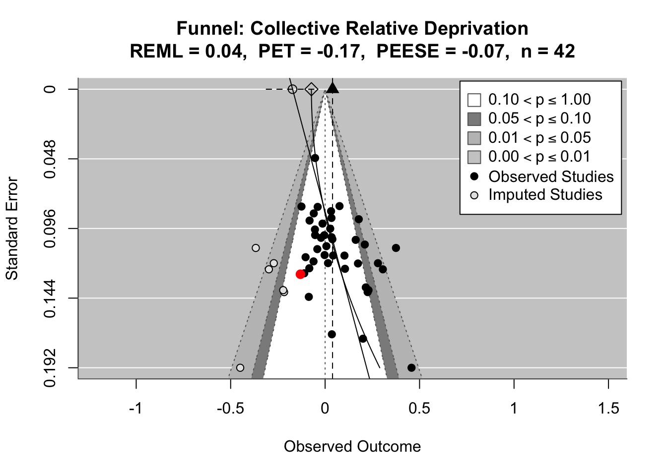
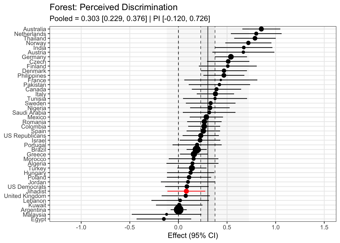
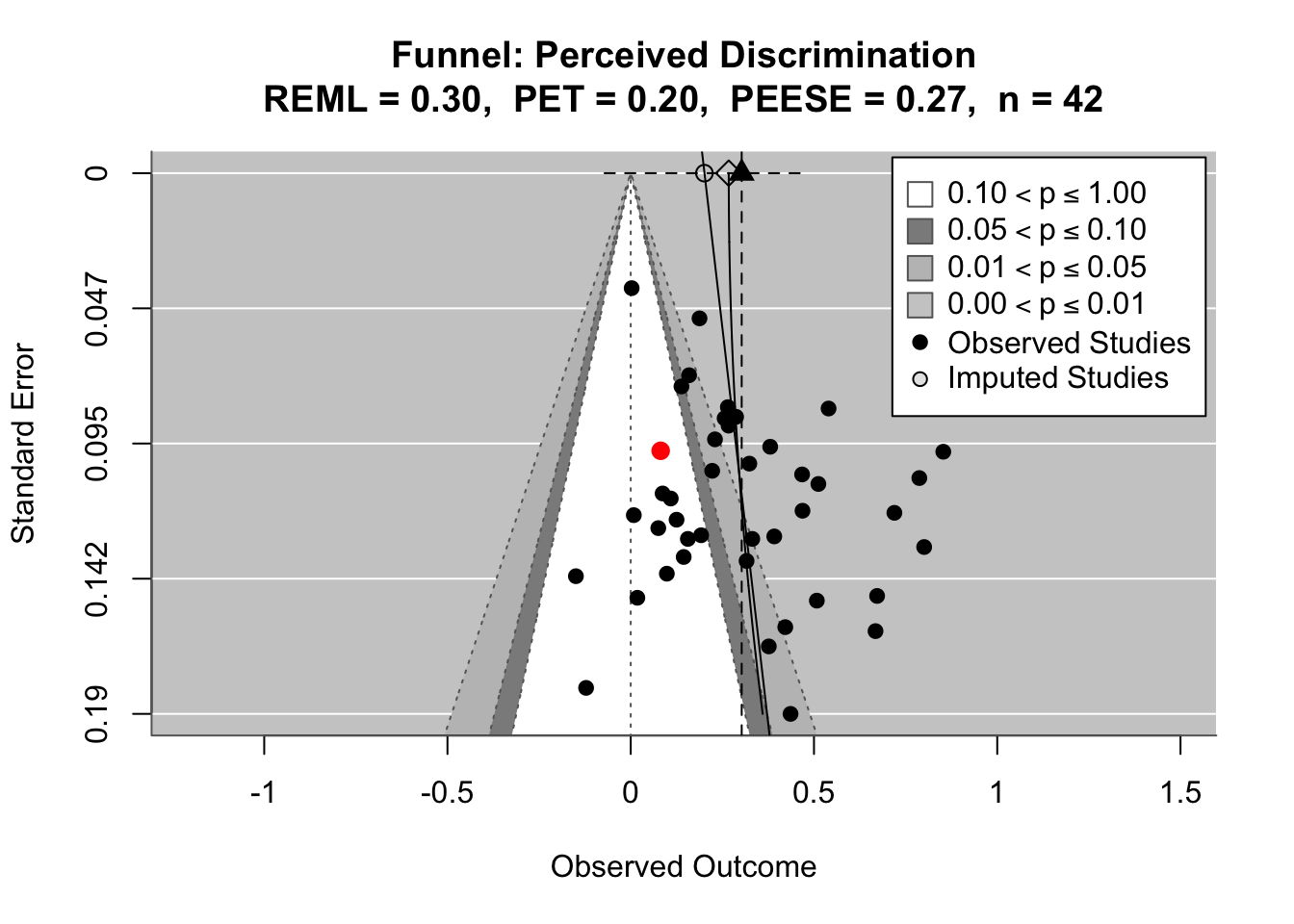
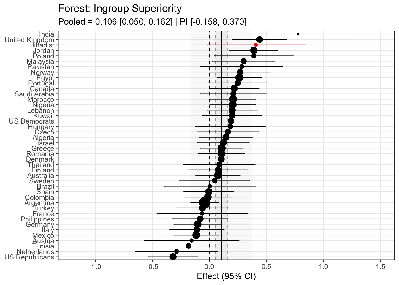
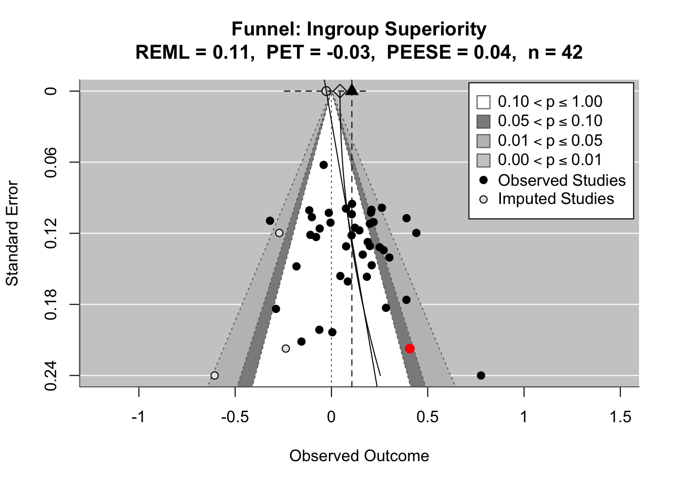
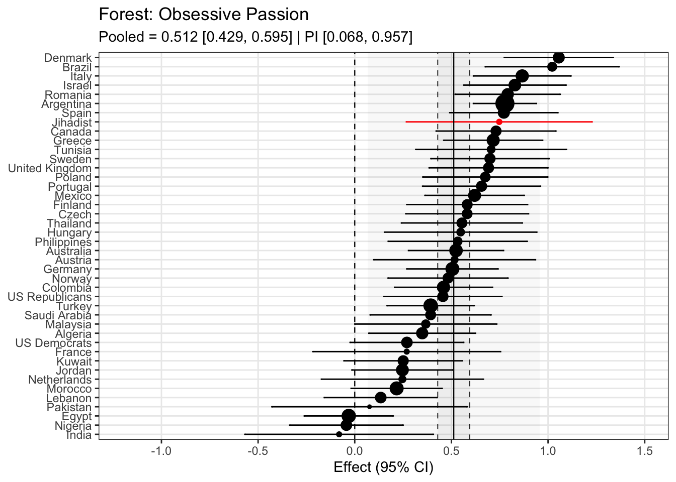
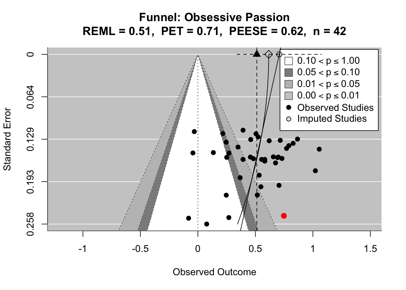
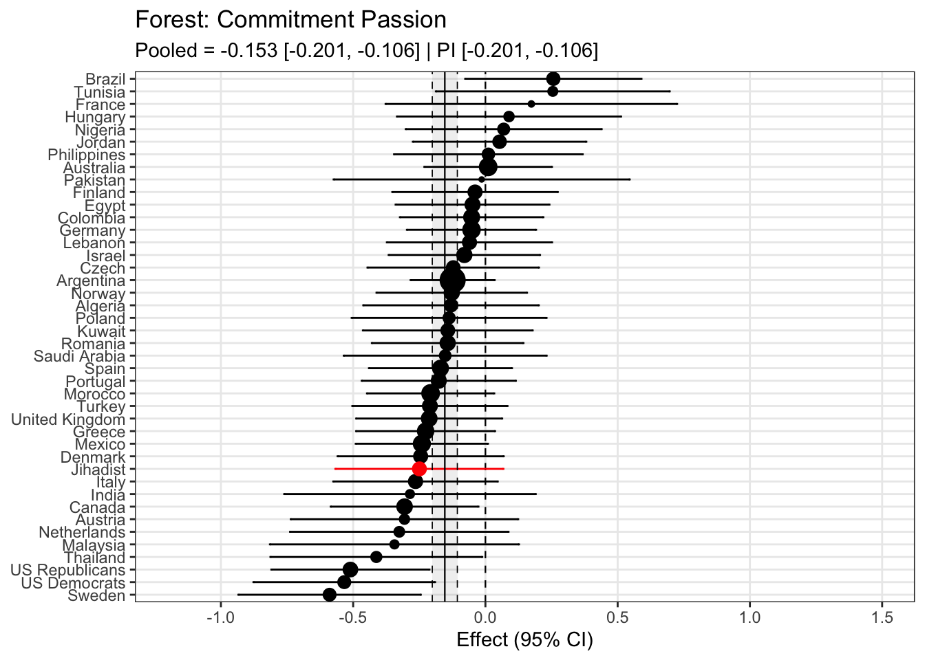
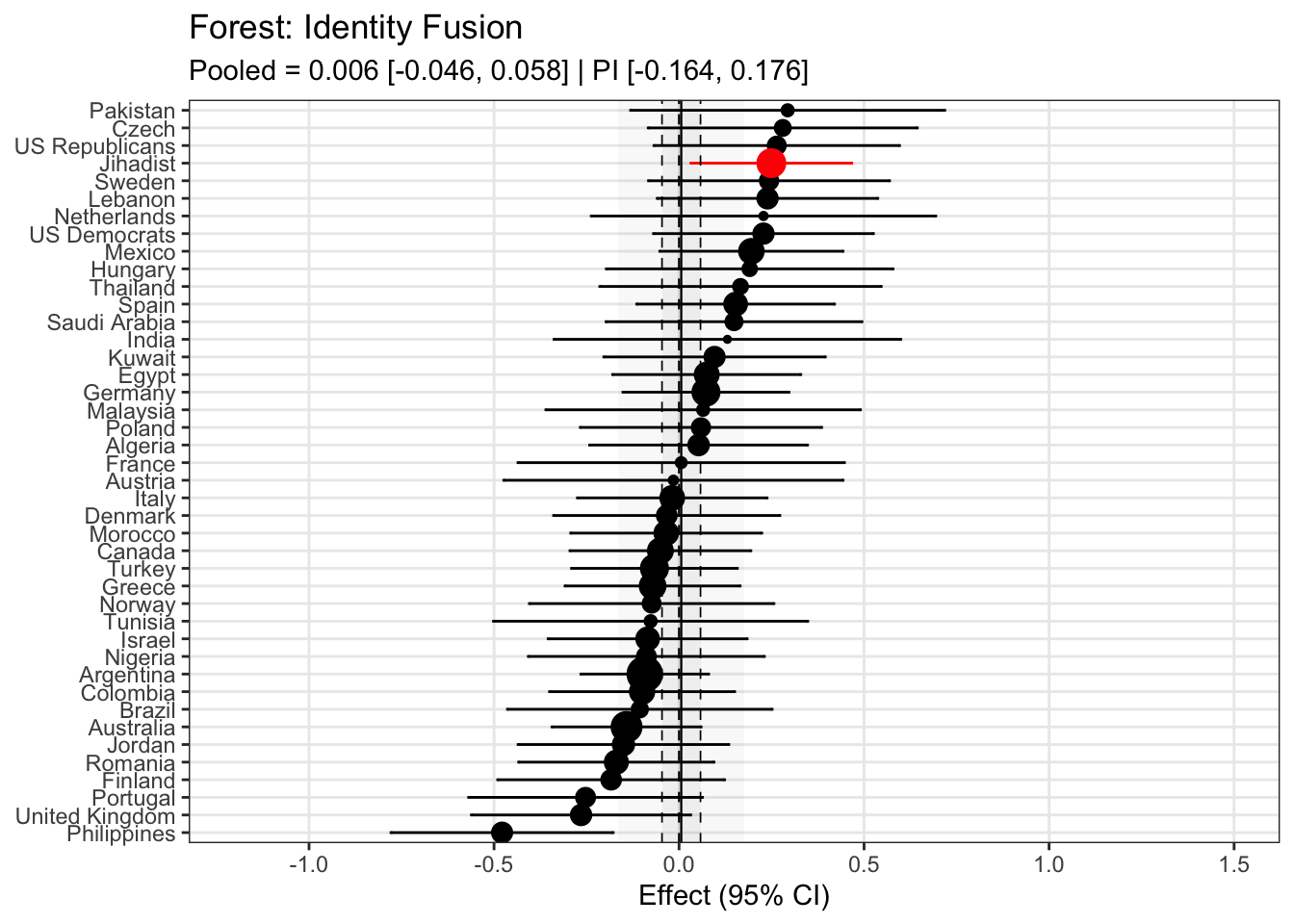
To compare effects across countries transparently, we refitted the same country-level linear model using grand-mean standardized predictors (suffix _gmz), extracted per-country coefficients and standard errors. We now meta-analyze them with a random-effects model (REML). This yields an overall average effect and heterogeneity statistics (Q, τ², I²).
Code
meta_results <- country_effects %>% tidyr::nest(data =c(country, estimate, std.error)) %>%# one row per term dplyr::mutate(.results = purrr::map(data, ~ metafor::rma(yi = .x$estimate,sei = .x$std.error,method ="REML",slab = .x$country )) ) %>% dplyr::select(term, .results)